Chapter 5 Basic regression analysis
5.1 Introduction
The first chapters of the course covers what we may call “basic statistics”. We will now take up regression analysis . In general, regression analysis provide us with methods to study and analyze relations and interactions between random variables. Needless to say, the study of such relations is fundamental to any form of applied science. In economics, business administration, logistics and supply chain management one continuously deals with different variables and how they may affect each other. Regression analysis is the tool that may take us from guessing to knowing in such contexts. In this chapter we will consider relations between only two variables. Later the case where many variables simultaneously affect another variable will be discussed.
5.1.1 A motivating example
The introduction above is written in general terms. Let us consider a very specific example where two random variables are related.
In chapter 4.5, we discussed a data file from a transportation company. Part of the data looks as seen below. The objects in the data file are a set customer to customer trips. For each trip, the variable Duration represent the time taken to go from customer A to B, while the variable Distance represents the actual traveling distance from A to B.
#read data
trips <- read.csv("Data/Trip_durations.csv")
#An alternative is
#look at top rows, and a summary of the duration variable:
head(trips)
## Duration Distance
## 1 12.5 2.74
## 2 33.5 13.60
## 3 33.1 10.99
## 4 37.0 10.31
## 5 18.3 4.93
## 6 29.3 8.15To simplify notation, let us call the variables \(Y\) and \(X\), with \(Y\) being the duration of the trip, \(X\) being the distance. Now, we would clearly expect a relation between the variables \(X\) and \(Y\). Quite obviously, we would expect longer distance trips to take longer time. In other words, we would expect positive correlation between the two variables. With our R knowledge, we can easily compute the correlation coefficient. It is \[ r_{xy} = 0.946\;. \]
## [1] 0.9461513In basic economics and other subjects, relations between variables are commonly represented by functional relations i.e. one puts up a model like \[ y = f(x)\;, \] where the variable \(y\) is some exact function of the variable \(x\).
For instance, one could propose a linear relation between the duration and the distance, to get the functional relation \[ y = a + bx\;. \] This model represents two assumptions, (i) - that the relation is actually linear, and (ii) - that the relation is deterministic. The second assumption means that for a given distance \(x\), we may predict with 100% accuracy the duration of the trip. Common sense tells us that this assumption is not valid. We know that trips of a given distance \(x\), may result in somewhat variable durations, due to other factors. It means we should add some randomness to the model, to make it more realistic. A scatterplot of the relation is shown in figure 5.1. We see the clear dependency, that longer distance trips tend to give longer durations. Even though the dependency is quite strong, there is also a bit of “randomness”. It appears impossible to exactly predict the durations of a trip of 10 km distance. There are some 12 km trips with shorter duration than some of the 8 km trips. How can we model the relation in a more realistic way?
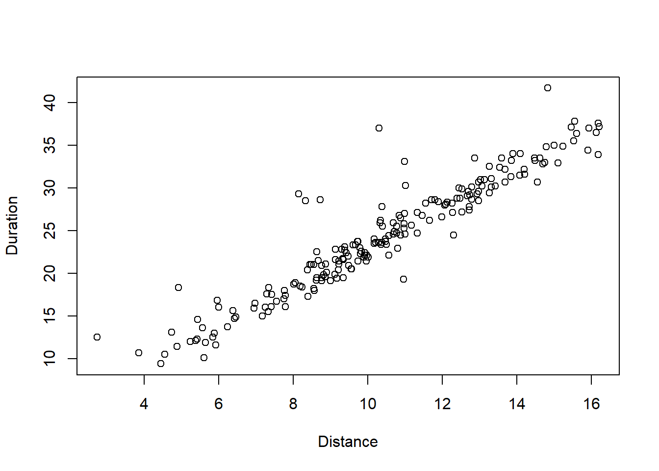
Figure 5.1: A scatterplot.
We need to move from a deterministic functional relation to a statistical functional relation This means we would describe the dependency by \[ Y = f(X) + \mathcal{E};.\] This means \(Y\) is the sum of a deterministic function of \(X\) plus a random variable \(\mathcal{E}\). The random variable represents all other factors that may affect \(Y\) in addition to the distance \(X\), as for instance traffic intensity, speed limits and so on. The function \(y = f(x)\) represents the average effect of distance on duration. We often speak about the trend when talking about \(f(x)\). In the scatterplot in figure 5.1, we would say that we see something close to a linear trend, i.e. that the function \(f(x)\) should be linear (or close to that). If we believe in a linear trend, our model would be \[\begin{equation} Y = a + bX + \mathcal{E}\;, \tag{5.1} \end{equation}\] meaning that on average, a trip of distance \(X\) will have a duration given by \(Y_{mean} = a + bX\), while each individual trip of distance \(X\) will be affected by some random deviation from \(Y_{mean}\).
The equation written in (5.1) is an example of a general linear two - variable regression model. It describes how we conceive the relation between the two variables \(X\) and \(Y\). The numbers \(a, b\) are parameters to the model. The primary task in regression analysis is to estimate such parameters, given a data material as seen in this example. The estimates will be specific numerical values for \(a, b\) giving the “most correct” linear trend given the data. In this particular case, R gives the estimated linear trend \[\begin{equation} y = 1.16 + 2.23x \;. \tag{5.2} \end{equation}\] We call this the estimated model. (We will soon se how to use R to obtain such estimates). Equation (5.2) gives a concrete description of the relation between \(X\) and \(Y\). This means the company would forecast a duration \(y\) of a trip with \(x = 10\) km as follows. \[ y = 1.16 + 2.23 \cdot 10 = 23.46\;. \] Another more general understanding coming from the estimated model, is that each additional km of distance on average adds approximately 2.23 minutes to the duration. Even such very basic use of regression analysis can be valuable, for instance in the operational planning for a transport company.
In figure 5.2, we see the scatterplot for the duration/distance data, along with the regression line, corresponding to the estimated linear model. It is simply the line with the equation in (5.2). Such figures can easily be provided by R. Detailed code will be shown shortly, after we get the basic theoretical ideas here.
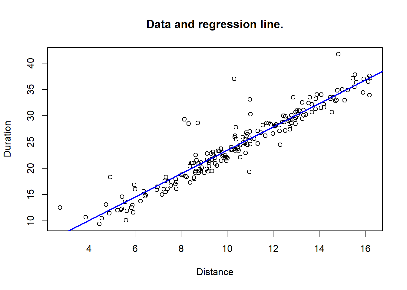
Figure 5.2: Data with fitted regression line.
With this example as background, let us take a general view on regression with two variables.
5.2 The linear two-variable model
Suppose we are interested in analyzing a possible linear statistical relation between variables \(X\) and \(Y\). In general we will use the formulation \[\begin{equation} Y = \beta_0 + \beta_1 X + \mathcal{E} \tag{5.3} \end{equation}\] of the model, i.e. the parameters of the linear trend are written \(\beta_0, \beta_1\). The parameters are often called regression coefficients. The first goal in a regression analysis is to obtain estimates for the parameters, based on a set of observations (data) \[ (x_1, y_1), (x_2, y_2), \ldots, (x_n, y_n) \] of corresponding \(X\) and \(Y\) values.
The following terminology is commonly used in regression models. The \(Y\) variable is called the dependent variable, while \(X\) is called the independent variable. Sometimes you will also see the \(X\) variable called a predictor variable. The latter name comes from the fact that in regression analysis, \(X\) values are typically used to predict (forecast) \(Y\) values.
The regression model in (5.3) also involves a third parameter which is the standard deviation \(\sigma_e\) of the random term \(\mathcal{E}\). This parameter describes how large deviations in \(Y\) values we are likely to see (away from the straight line). A small \(\sigma_e\) corresponds to a strong linear relation, with points close to the regression line. A larger \(\sigma_e\) means “more randomness”, so the linear pattern will be less evident in a scatterplot.
Remark on notation. When dealing with regression analysis, we usually think of the variables as random variables. When thinking like this, we try to use capital letters, e.g. \(X, Y\). On the other hand, when we work with the estimated linear trend, for instance, this is a deterministic relation, so we write this with smallcap letters, e.g. \(y = a + bx\). We will sometimes need to stress the fact that the pair of variables \((X, Y)\) will be observed \(n\) times, and that each observation for \(i = 1, 2, \ldots, n\) involves distinct random variables, but with the same distributions and governed by the same functional relation. In case of linear regression, we would then write the model in (5.3) as \[ Y_i = \beta_0 + \beta_1 X_i + \mathcal{E}_i \;, \quad \mbox{for $i = 1, 2, \ldots, n$}.\] This formulation means the same as the original, but it stresses the fact that for each new observation of \((X_i, Y_i)\) there is a distinct error term \(\mathcal{E}_i\).
Let’s see an example of some further possible applications of regression models. Note that we have no guarantee that any of these example would fit with a linear model.
:::{.example, #applications-simple name=“Applications of regression models.”}
- Real estate market: \(Y\) = price of a house, \(X\) = size in square meters.
- Production system: \(Y\) = processing time of a part, \(X\) = the number of holes to be drilled.
- Forestry: \(Y\) = usable volume of wood in a tree; \(X\) = the diameter at ground level.
- Economics: \(Y\) = demand for a product, \(X\) = price of product.
- This is typically a nonlinear relation, i.e. \(Y = f(X) + \mathcal{E}\), where \(f(x)\) is a non-linear function.
- Weather: \(Y\) = flow of water in the Molde river, \(X\) = amount of rain for the last 48 hours.
- Transport: \(Y\) = duration of a delivery route, \(X\) = number of deliveries.
:::
5.2.1 Theoretical vs estimated linear model
Consider the linear model \[ Y = \beta_0 + \beta_1 X + \mathcal{E}. \] with its three parameters: \(\beta_0, \beta_1\) and \(\sigma_e = \mbox{Sd}{[\mathcal{E}]}\). We call this the theoretical model. This represents our assumptions of the structure of the relation between \(X\) and \(Y\). The true parameter values will never be known exactly. On the other hand, using data, we can estimate the best fitting linear model, \[ Y = b_0 + b_1 X, \] where \(b_0, b_1\) are specific numbers, estimates of the true parameters. This equation is what we call the estimated model. Another name is simply the regression line (fitted to a particular data set). An estimate for \(\sigma_e\) can also be made, along with the coefficient estimates.
In general, it is the estimated model that we can use in practice - to make forecasts and predictions - and to somehow quantify the relation between the two variables. Note, however: If the theoretical model is not close to a correct description of reality, the estimated model will give false conclusions about the reality we study. For instance, if the real relation between variables is non-linear, and we use a linear model, we are likely to get a useless estimated model.
5.2.2 Model assumptions
The application of regression analysis requires certain assumptions on the model components to hold. We consider the linear model formulated by \[ Y_i = \beta_0 + \beta_1 X_i + \mathcal{E}_i \;, \] as explained in the remark above. With this formulation, we can state the basic model assumptions.
A. The data \((X_i, Y_i)\) represent a random sample from the population we study.
B. The error terms all have the same normal distribution with \(\mbox{E}{[\mathcal{E}_i]} = 0.\)
C. The error term is statistically independent of \(X\).
D. For all \(i\), the standard deviation is the same, \(\mbox{Sd}{[\mathcal{E}_i]} = \sigma_e\).
Assumption A means that the objects we study (e.g. houses, persons) are selected randomly from a larger population, and then \(X_i, Y_i\) are observed. Assumption B limits the methods to situations where error terms are (close to) normal. Assumptions C means that for any observation pair, the \(\mathcal{E}\) value is equally likely to be positive and negative, and on average the error is 0, regardless of the \(X\) value. Assumption D states that the size of errors (deviations) is uniform over the range of possible \(X\) values.
5.2.3 Parameter estimation for the linear model
The parameter estimates based on a set of observations \[ (x_1, y_1), (x_2, y_2), \ldots, (x_n, y_n) \] comes from what is known as the least squares method. It is a fairly simple idea. We are looking for a particular line \[ y = b_0 + b_1 x \] that fits best with the trend shown by the \(n\) data points. Ok, so for any suggested line, say \[ y = a_0 + a_1 x \] we define the square sum of error (\(SSE\)) as follows. For each observed \(x_i\), let \(\hat{y}_i\) be the model prediction using the suggested line, i.e. \[ \hat{y}_i = a_0 + a_1 x_i\;. \] Now, the idea is that if the suggested line roughly follows the actual observed points \((x_i, y_i)\) in the scatterplot, most of the deviations \[ e_i = \hat{y}_i - y_i \] will be fairly close to 0, and consequently the squares \(e^2_i\) will be small (and positive). On the other hand, if the suggested line makes a poor fit with observed data, many of the deviations \(e_i\) will be far from 0, and consequently many of the squares \(e^2_i\) will be relatively large.
Now, to make a total measure of how well a given line \[ y = a_0 + a_1 x \] fits to the particular data, we simply sum all the square deviations \(e^2_i\), i.e we define \[ SSE = \sum_i e_i^2\;. \] We then simply select the line which has the minimal value for \(SSE\) to be the “best fitted line” for the given data. The numbers \(e_i\) coming from the estimated model are called residuals. We can say that we want the line giving overall the smallest possible residuals.
Looking at a figure should clarify the method completely. In figure 5.3, we once again see the scatter plot for durations/distance data. Two possible lines are drawn. The red one is \[ y = 30 - 0.9x \] and the blue one is \[ y = -1.6 + 2.5 x \;. \]
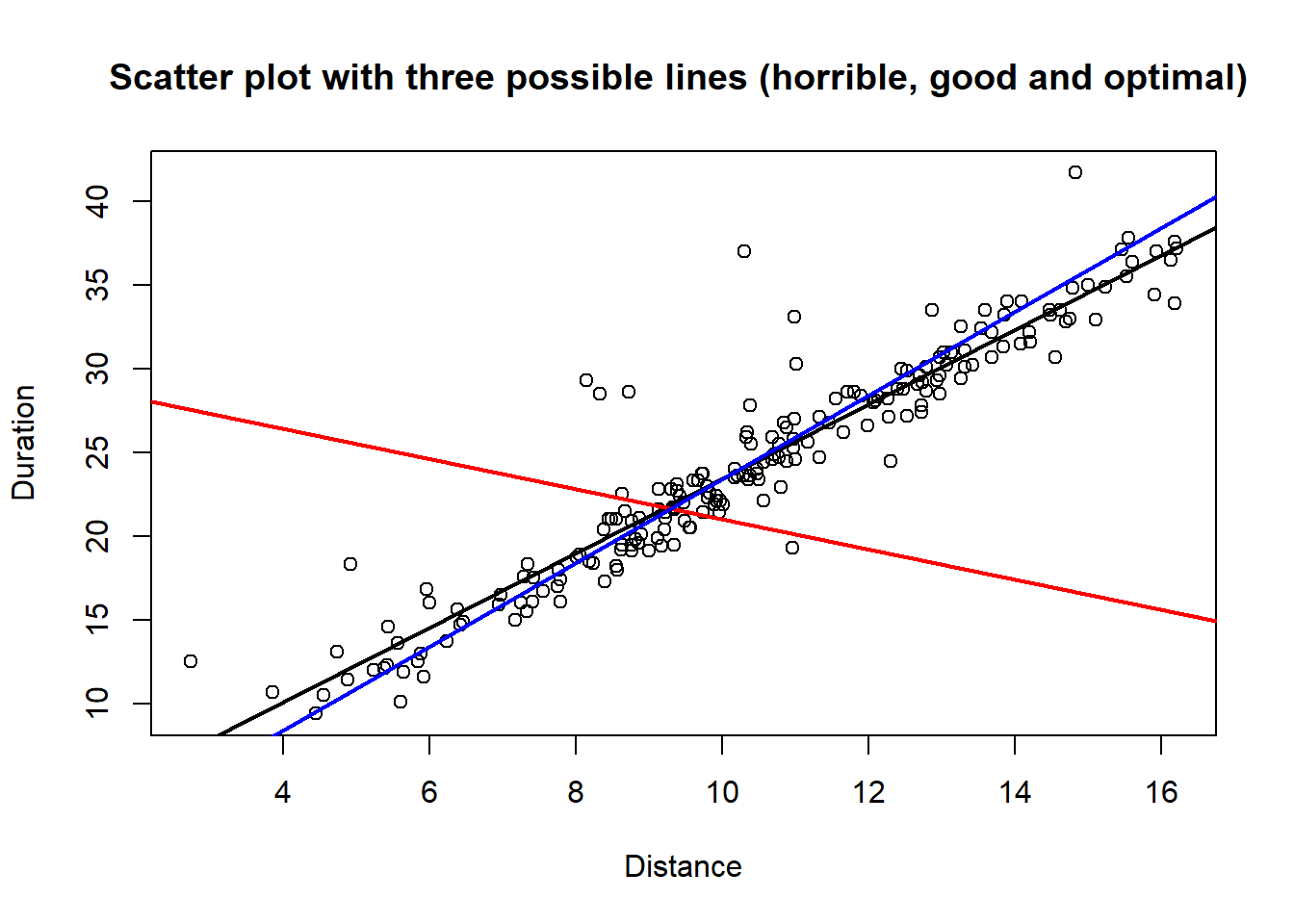
Figure 5.3: Three lines with variable degree of fit to data.
We see that for almost any \(x_i\) value, the blue line gives a corresponding \(\hat{y}_i\) value much closer to the observed \(y_i\) value, than what we get from the red line. Thus, the SSE value for the blue line is much lower than for the red line, and the blue is apparently a much better fit to data. Still better is the actual regression line, shown in black. It should be understood that the minimization of SSE that leads to the regression line is done by R, and not something we need to worry about in terms of calculations. For us it is sufficient to have an idea what it is that defines the particular line we want.
5.3 Using R in regression
Let’s pause the theoretical development to see how we run a regression analysis with R. We continue working on the duration/distance data.
In R we will always have our data in a data frame, in this case it is called trips and we can review a quick look at the data.
##   Duration Distance
## 1     12.5     2.74
## 2     33.5    13.60
## 3     33.1    10.99
## 4     37.0    10.31
## 5     18.3     4.93
## 6 29.3 8.15So we have columns Distance and Duration which are our \(X\) and \(Y\) variables in this case. In other words, Duration is the dependent variable, Distance is the independent variable. To run a regression with the linear model here, we use a code like
This creates a regression object here called myreg. This is a special object that contains a lot of information about the regression model estimated. We have several functions that present results from this analysis. For starters, we can look at coef and summary. The function coef prints just the estimated coefficients.
## (Intercept)    Distance
##    1.162025    2.225569
Much more information (we will explain most of this later) is given by summary.
##
## Call:
## lm(formula = Duration ~ Distance, data = trips)
##
## Residuals:
##     Min      1Q  Median      3Q     Max
## -6.2543 -1.1549 -0.2876  0.7293 12.8924
##
## Coefficients:
##             Estimate Std. Error t value Pr(>|t|)
## (Intercept)  1.16202    0.58432   1.989   0.0481 *
## Distance     2.22557    0.05412  41.126   <2e-16 ***
## ---
## Signif. codes:  0 '***' 0.001 '**' 0.01 '*' 0.05 '.' 0.1 ' ' 1
##
## Residual standard error: 2.218 on 198 degrees of freedom
## Multiple R-squared:  0.8952, Adjusted R-squared:  0.8947
## F-statistic:  1691 on 1 and 198 DF,  p-value: < 2.2e-16
The rows labeled (Intercept) and Distance contain information on the estimates \(b_0\) and \(b_1\) respectively.
For now we concentrate on the column Estimate which gives the actual estimated values. These are as we see about
1.16 and 2.23.
As previously seen, the regression line
then becomes
\[ y = b_0 + b_1 x = 1.16 + 2.23 x \;.\]
Remember that the numbers \(b_0, b_1\) are estimates. They are never equal to the true parameter values \(\beta_0, \beta_1\). The uncertainty
of the estimates are reflected in the two numbers in the column Std. Error.
As in all statistics, a fundamental question will be:
how close are the true parameter values to the estimates \(b_0, b_1\). The answer to such questions are given by confidence intervals.
We next turn to such issues, but firstly we show how to plot the data along with the regression line. Recall that myreg was the regression object. The abline function can be used in different ways to draw straight lines, and if we use it with a (simple) regression object, it will draw the estimated line into a given plot. Like this:
#plot observed data:
with(trips, plot(Distance, Duration, main="An example regression plot."))
#add regression line: (color blue, line width = 2)
abline(myreg, col = "blue", lwd = 2)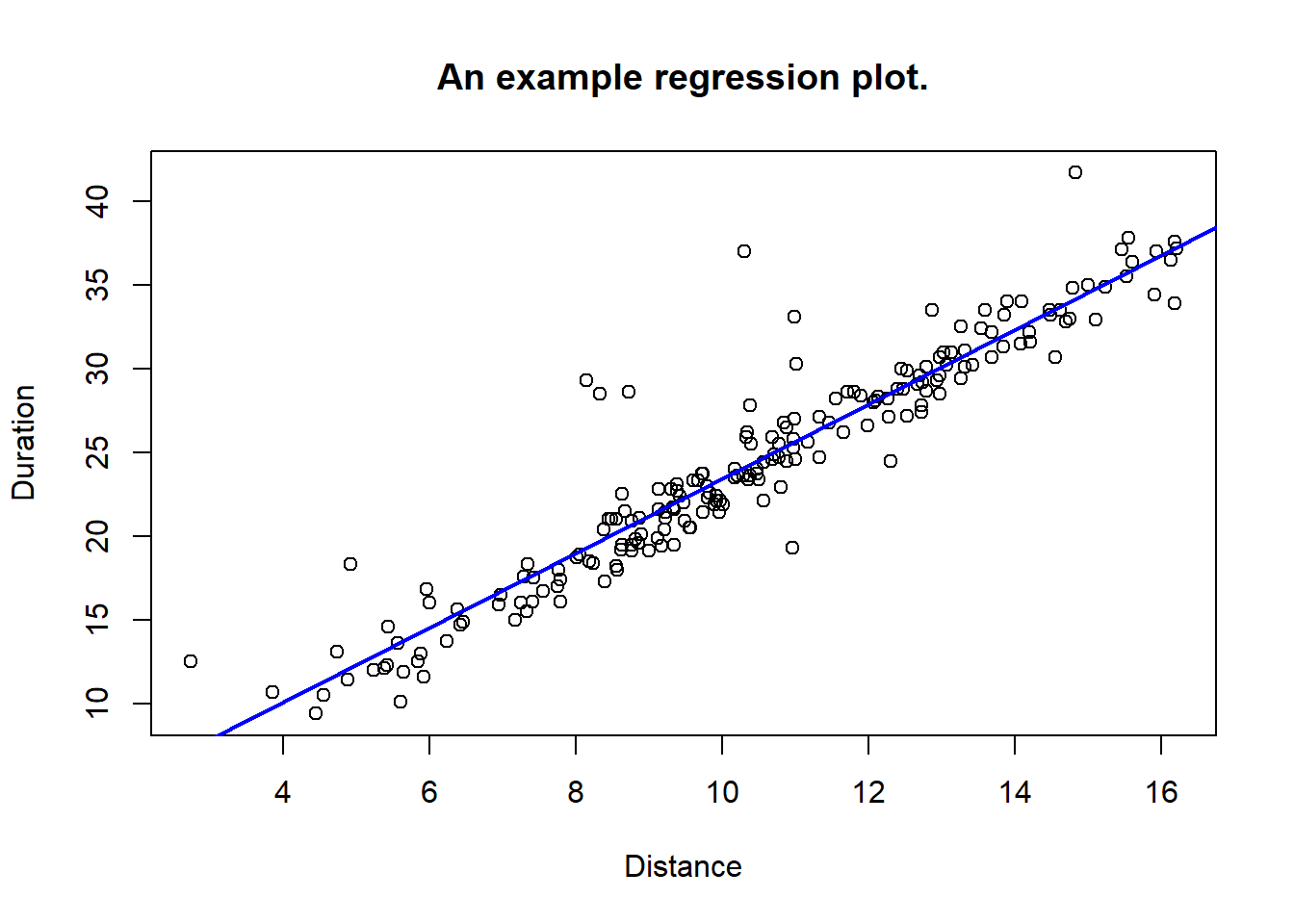
5.4 Inference in regression analysis
Let’s repeat the main business of statistics: Sample-based statistics leads to estimates for certain parameters. Inference simply means to go from sample information (estimates) to statements about parameters. There are two main forms of statements about parameters in statistics:
Confidence intervals: E.g “with 99% confidence, \(\mu\) is between \(A\) and \(B\).”
Conclusions to hypothesis tests: E.g. “we reject the null hypothesis \(p = 0.20\) in favor of the alternative \(p \ne 0.20\) with significance level \(\alpha = 0.05\).”
In this section, we show how we can come to such inference statements about the two regression coefficients \(\beta_0, \beta_1\). This will be of great importance. If we only know that the estimated regression line is given by (say) \[ y = 23.6 + 2.35 x\;, \] this can not be used properly for making decisions. We must have knowledge of how reliable the estimates are, if we want to make important decisions based on an estimated regression model. Therefore - inference statements are indispensible. Furthermore, we will see that inference statements are quite easy to obtain in regression, using R and a little bit of theory.
5.4.1 Sampling distribution for \(b_i\)
The theoretical result that makes inference in regression analysis work, is as follows. Of course, this is only valid if the basic assumptions for using regression are satisfied. Then, we consider the theoretical model \[ Y = \beta_0 + \beta_1 X + \mathcal{E} \] and let \(b_0, b_1\) be the coefficient estimates based on the least squares method. Considering \(b_0, b_1\) as random variables, let \[\begin{equation} S_{b_0}, S_{b_1} \tag{5.4} \end{equation}\] be the standard deviations. Then if \(n\) denotes the sample size, \(\beta_i, i = 0, 1\) are the true parameters, we find that \[\begin{equation} T = \frac{b_i - \beta_i}{S_{b_i}} \tag{5.5} \end{equation}\] has a \(t\) distribution with \(DF = n - 2\). This result allows us to compute confidence intervals and to test hypotheses about the \(\beta_i\) parameters.
5.4.2 Confidence intervals
Using the sampling distribution result above, we can find the following formula for a \((1 - \alpha)\cdot 100\) % confidence interval for \(\beta_i\). \[\begin{equation} b_i \pm t^{^{n-2}}_{_{\alpha/2}} S_{b_i} \tag{5.6} \end{equation}\] Here, the \(t^{^{n-2}}_{_{\alpha/2}}\) is the particular value cutting off probability \[ \alpha / 2 \] to the right, for the \(t\) distribution with \(DF = n-2\). (Similar to the \(z_{_{\alpha/2}}\) we used for standard normal distribution.) At the moment, it is probably not clear how to use the formula in (5.6). We need to know how to find the input numbers from R. We will come back to this shortly, but first we discuss the very much related issue about hypothesis testing.
5.4.3 Testing hypotheses about regression coefficients.
In every regression analysis, there are two particularly important hypotheses that we should test. It concerns the possible situation that a true coefficient \(\beta_i\) is equal to 0. Since all estimates are based on a random sample, even if \(\beta_1 = 0\), we will never exactly observe \(b_1 = 0\). Random effects in the sample will lead to an estimate somewhat different from 0. In practice, we never see \(\beta_1\), but we see \(b_1\). If the \(b_1\) value does not convince us that \(\beta_1 \ne 0\), we really have no strong indication that the \(X\) variable affects \(Y\) in a linear relation. To realize this, just write the model, with \(\beta_1 = 0\). It becomes \[ Y = \beta_0 + 0\cdot X + \mathcal{E} = \beta_0 + \mathcal{E} \;, \] and we see the whole relation between the variables disappear. So, if we can not reject the hypothesis that \(\beta_1 = 0\) - our whole regression analysis breaks down. We should not try to analyze a relation which with good probability does not exist!
Note that the corresponding situation with the other parameter, \(\beta_0\) is not that serious. If \(\beta_0 = 0\), it just means that the relation between \(X\) and \(Y\) is linear without a constant term, i.e. it is \[ Y = \beta_1 X + \mathcal{E} \] and it still makes sense to analyze the relation.
We focus now on the parameter \(\beta_1\). More formally, we set up the hypothesis test as follows. \[\begin{equation} H_0: \beta_1 = 0 \ \mbox{vs.} \ H_1: \beta_1 \ne 0 \;. \tag{5.7} \end{equation}\]
The test statistic will be \[ T_{b_1} = \frac{b_1}{S_{b_1}}\;, \] and the null distribution is a \(t\) distribution with \(n-2\) degrees of freedom. The procedure of the test is the usual one: The sample observations lead to an observed value \(T_{_{OBS}}\). Then one can compute the P-value, which - as you hopefully recall - is the probability of seeing a value for \(T\) that is more critical than \(T_{_{OBS}}\). Typically, one uses the significance level \(\alpha = 0.05\). We shall usually use R to compute the P-value for us, so we only need to check: If the P-value is less than 0.05 - we reject \(H_0\). We call this the standard coefficient test in regression analysis. A perfectly similar test can be done for the \(\beta_0\) parameter, with the test statistic \[T_{b_0} = \frac{b_0}{S_{b_0}}\;. \]
Building on the same idea, in a regression application we are often interested in testing a more general hypothesis about the coefficients, say a two-sided test \[\begin{equation} H_0: \beta_1 = \beta^* \ \mbox{vs.} \ H_1: \beta_1 \ne \beta^*\;, \tag{5.8} \end{equation}\]
where \(\beta^*\) is some constant. In this case we look back to (5.5). Given that \(H_0\) is true, the \(T\) value becomes \[\begin{equation} T = \frac{b_1 - \beta^*}{S_{b_1}}\;. \tag{5.9} \end{equation}\] From the results in section 5.4.1 we know that this \(T\) statistic will have the given \(t\) distribution with \(n-2\) degrees of freedom, and this is what we need to know to be able to compute P-values. We realize that the standard hypothesis test in (5.7) corresponds to the general test with a two-sided alternative, when \(\beta^* = 0\). The next section outlines how these theoretical inference results relates to R regression output.
5.4.4 Regression inference with R
Let us see how we can work on inference issues in regression when using R. We continue using the durations/distance example.
Suppose we run regression as in section 5.3 using the lm function and obtain the regression object myreg.
The basic confidence intervals from (5.6) can be obtained by the built-in function
confint as follows.
##                   2.5 %   97.5 %
## (Intercept) 0.009744218 2.314305
## Distance    2.118851576 2.332286
We see that for the \(\beta_1\) parameter, the confidence interval is about [2.12, 2.33], meaning that the estimate \(b_1 = 2.23\) can be said to be relatively precise. The constant comes with more uncertainty, as we see from the wider confidence interval.
Let’s look again at the summary of the regression.
##
## Call:
## lm(formula = Duration ~ Distance, data = trips)
##
## Residuals:
##     Min      1Q  Median      3Q     Max
## -6.2543 -1.1549 -0.2876  0.7293 12.8924
##
## Coefficients:
##             Estimate Std. Error t value Pr(>|t|)
## (Intercept)  1.16202    0.58432   1.989   0.0481 *
## Distance     2.22557    0.05412  41.126   <2e-16 ***
## ---
## Signif. codes:  0 '***' 0.001 '**' 0.01 '*' 0.05 '.' 0.1 ' ' 1
##
## Residual standard error: 2.218 on 198 degrees of freedom
## Multiple R-squared:  0.8952, Adjusted R-squared:  0.8947
## F-statistic:  1691 on 1 and 198 DF,  p-value: < 2.2e-16
Now consider the two rows below “Coefficients:”
We see the basic coefficient estimates to the left, in the column Estimate. The next column labeled Std. Error
contains the standard deviations (\(S_{b_i}\)) of the estimators, the same as we
discussed around equation (5.4).
Moving to the next column, labeled t value, we find observed values for our test statistics. We see the values
\[ T_{b_0} = 1.989, \quad T_{b_1} = 41.13\;. \]
Just to make sure, we can check that the values match, for instance, we get
\[ T_{b_1} = \frac{b_1}{S_{b_1}} = \frac{2.226}{0.054} = 41.13 \]
The data set in this case has \(n = 200\), so the \(t\) distribution with \(DF = n - 2\) will be very close to standard normal.
Regarding the test of
\[ H_0: \beta_0 = 0 \ \mbox{vs.} \ H_1: \beta_0 \ne 0 \;, \]
we find the P-value at 0.048, and thus we reject \(H_0\) with quite weak evidence. On the other hand, the test for \(\beta_1\) gives
a P-value at 0.000, so we can reject the hypothesis \(\beta_1 = 0\) with very strong evidence. (The extremely low P-value corresponds to the extreme \(T_{_{OBS}}= 41.13\), We see that R only puts the value lower than \(2\cdot 10^{-16}\) which is indeed close to 0.).
So, as a preliminary summary of the analysis, it appears (unsurprisingly) that there is a strong relation between a trips distance and the duration. There is a small constant contribution to the duration estimated at 0 to 2.3 minutes. The coefficient \(\beta_1\) represents the added duration per added kilometer of distance to a trip. It is estimated to lie in the interval 2.12 to 2.33 minutes. It means for instance that if the transport company make their plans under the assumption that \(\beta_1 < 2.5\), they are very likely to be on the safe side.
We can also investigate the question whether \(\beta_1 < 2.5\), using the general coefficient test from (5.8) with a one-sided alternative and \(\beta^* = 2.5\), i.e. we test \[ H_0: \beta_1 = 2.5 \ \mbox{vs.} \ H_1: \beta_1 < 2.5\; \] The general \(T\) statistic is \[T = \frac{b_1 - 2.5}{S_{b_1}} = \frac{2.226 - 2.5}{0.054} = - 5.07\;. \] We note that the \(T\) value is on the critical side of 0 for this test, and using an \(N(0, 1)\) approximation, we see that the P-value for the test is practically 0. We reject the null hypothesis and conclude with high confidence that \(\beta_ 1 < 2.5\).
Suppose we have a situation where we want to estimate a linear regression model \[ y = b_0 + b_1 x \] based on a data material \[ (x_1, y_1), (x_2, y_2), \ldots, (x_n, y_n)\;. \] We now show how we can use the data to split the observed variation in the \(y\)-data in two components. In a regression setting, there are two sources of variation in the \(y\) variable:
A Dependency on the \(x\) variable. When \(x\) varies, \(y\) varies because it is partly dependent on \(x\). B. Randomness. There is a random element in every \(y\) observation. (Otherwise \(y\) would be completely determined by \(x\).)
It is possible to compute two measures from data to find the relative contributions of each of the sources A and B. For A, it is called \(SSR\), the Square sum of Regression. For source B, it is called \(SSE\), the Square Sum of Error. We can then obtain the Square sum of Total variation, \(SST\) by \[\begin{equation} SST = SSR + SSE\;. \tag{5.10} \end{equation}\] Now, there are two central uses of these square sums.
Firstly, the ratio \[ \frac{SSR}{SST} \] shows exactly how much of the total variation in \(y\) can be attributed to the dependency of \(x\). So the ratio becomes a measure of how strongly \(y\) depends on \(x\). The ratio is called the \(R-square\) of an estimated regression model, and we write \[ R^2 =\frac{SSR}{SST}\;. \] The \(R^2\) is a number between 0 and 1, and a value close to 1 indicates a strong linear relation between the variables.
Secondly, the Square Sum of Error, \(SSE\) is directly linked to the sizes of deviations of \(y_i\) from the regression line. In fact, writing \[ \hat{y}_i = b_0 + b_1 x_i \] for the model predictions, we will simply have \[ SSE = \sum_{i = 1}^n (y_i - \hat{y}_i)^2 \;. \] It turns out (not surprisingly, maybe) that \(SSE\) is directly involved in an estimate for the third parameter, \(\sigma_e\), which is the standard deviation of the random term \(\mathcal{E}\) in the basic model. The actual estimate is \[\begin{equation} S_e = \sqrt{\frac{SSE}{n-2}} \tag{5.11} \end{equation}\] The \(S_e\) estimate is super-important in many practical regression applications, because it is telling us exactly how precise we can hope to be, when we try to use \(x\) values to forecast (predict) \(y\) values.
5.4.5 More about R regression: \(R^2\) and predictions
The numbers that we have now briefly discussed, can be obtained with R via the regression object as we will now see.
We can continue our Distance/Duration example further. Firstly, regarding the \(S_e\) estimate, look at the output from summary above. There we find the line Residual standard error: 2.218 .... This number is the \(S_e\) in this particular example.
Moreover, we find the line Multiple R-squared: 0.8952, ... This number is the \(R^2\) for the given regression.
If we would want to see the values for the square sums, we can use the anova function. It looks like this.
## Analysis of Variance Table
##
## Response: Duration
##            Df Sum Sq Mean Sq F value    Pr(>F)
## Distance    1 8323.6  8323.6  1691.4 < 2.2e-16 ***
## Residuals 198  974.4     4.9
## ---
## Signif. codes:  0 '***' 0.001 '**' 0.01 '*' 0.05 '.' 0.1 ' ' 1
So here the column Sum Sq gives respectively the \(SSR\) and the \(SSE\) for this regression. The \(SST\) is of course the sum of the two others. We can use the numbers just to verify that
\[R^2 = \frac{SSR}{SST} = \frac{8324}{8324 + 974} = 0.8952 \]
as calculated by R. We also verify that
\[ S_e = \sqrt{\frac{SSE}{n-2}} = \sqrt\frac{974.4}{198}=2.218 \]
The meaning of these numbers is as follows.
Since \(R^2\) is about 0.90, it means 90% of all the variation in trip duration (the \(y\) variable) can be explained by variation in trip distance (the \(x\) variable). It simply means that distance is a very strong determining factor for trip duration. That is hardly surprising, but now we have quantified the strength quite precisely.
Turning to the \(S_e\) value, at 2.22. What does this mean? Now, remember that our theoretical model states \[ Y = \beta_0 + \beta_1 X + \mathcal{E} \;. \] Also remember that we suppose \(\mathcal{E}\) to have a normal distribution with expected value \(\sigma_e\). That means, if we fix the value for \(X\), say \(X = x^*\), we will find the predicted \(Y\) value as \[ y^* = \beta_0 + \beta_1 x^* \] plus a normally distributed error, with standard deviation \(\sigma_e\). From our knowledge of normal distributions, we then know that with 95% probability, the \(Y\) value will be within \(2\sigma_e\) from the predicted value \(y^*\). Now, some readers will see that there are some problems to this. In fact, we do not know either of the values \(\beta_0, \beta_1, \sigma_e\). Provided the sample size is a bit large, say 30+, we can still use the idea here, just replacing all parameters with their estimates. So, our prediction is \[ y^* = b_0 + b_1 x^*\;, \] And we still find with good approximation: With 95% probability, the real \(Y\) value will be in the interval \[ y^* \pm 2 S_e \;. \] So, finally, since the SPSS output showed \(S_e = 2.22\), and \(n = 200\) in this case, we find a 95% margin of error for model predictions by \[ \mbox{ME}_{95} = 2 S_e = 4.44\;. \] So, trip distance allows a prediction of trip durations, but to be 95% sure, we must admit an error margin of about 4.44 minutes. If necessary, one can find more exact expressions for such margins of error. We will discuss those if we need to.
5.5 Graphical interpretation of the \(R^2\).
The \(R^2\) is a measure of how well an \(x\) variable works as a predictor for a \(y\) variable. The less randomness there is in the relation, the larger we find \(R^2\). In figure @ref(fig:four_r_squares) four scatterplots are shown. In the first plot, where \(R^2\) is about 0.98, we see that the \(y\) values are to a very high degree determined by the \(x\) value. In this case, for a given \(x\) value, we can predict the corresponding \(y\) value with only a small margin of error. In the last, where \(R^2 = 0.16\), we see \(y\) values varying almost independently of the corresponding \(x\) value. A given \(x\) value helps just a tiny bit to determine a corresponding \(y\) value. Predictions in this case must come with very high margins of error.
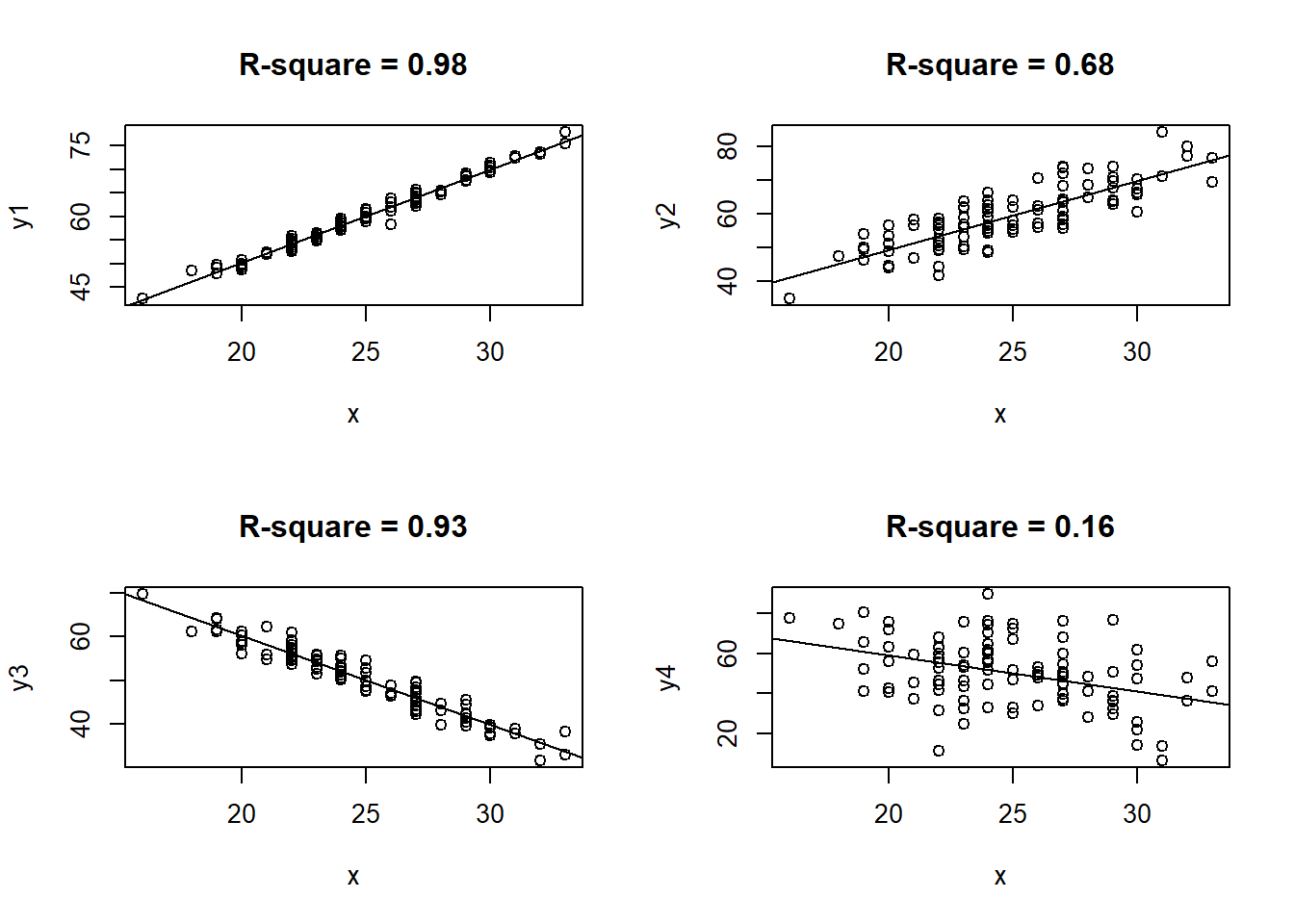
(#fig:four_r_squares)Four examples of \(R^2\).
5.6 Basic check of model assumptions
A thorough check of all regression model assumptions can be somewhat technical. In this section we only discuss the most basic steps we can do to assure that regression analysis can be validly applied to a data set. The basic model assumptions were listed in section 5.2.2, as assumptions A, B, C and D.
If you try to apply linear regression analysis to a pair of variables that are non-linearly related, you will see violations of more or less all the basic assumptions. To check linearity, a visual inspection of the scatterplot will normally be enough to reveal serious problems. Take a look at the example shown in figure 5.4. Apparently, there is a nonlinear structure in the relation between the two variables. Using R, there is nothing stopping us from fitting a line (e.g. a linear model), but clearly the model does not fit well with reality. Understanding that \(\mathcal{E}\) represents the deviations in the \(Y\) variable from the line, we see that for different values of \(X\), the deviations have very different distributions. We get a violation of (at least) assumptions B and C. For instance, the expected value of \(\mathcal{E}\) is for some \(X\) values clearly negative, for other \(X\) values it is clearly positive, violating assumption C. An estimated linear model will miss out much of the prediction power that the \(X\) variable has. Blindly running a linear regression will result in an \(R^2\) at about 0.90, so one may mistakenly accept the model as a fairly good predictive tool. It is not.
set.seed(1234)
s = 60.0
x <- runif(50,min = 10, max = 40)
err <- rnorm(50)
y = 15 + 0.02*x^3 + s*err
reg <- lm(y~x)

plot(x, y, main = "A nonlinear relation and a regression line.")
abline(reg)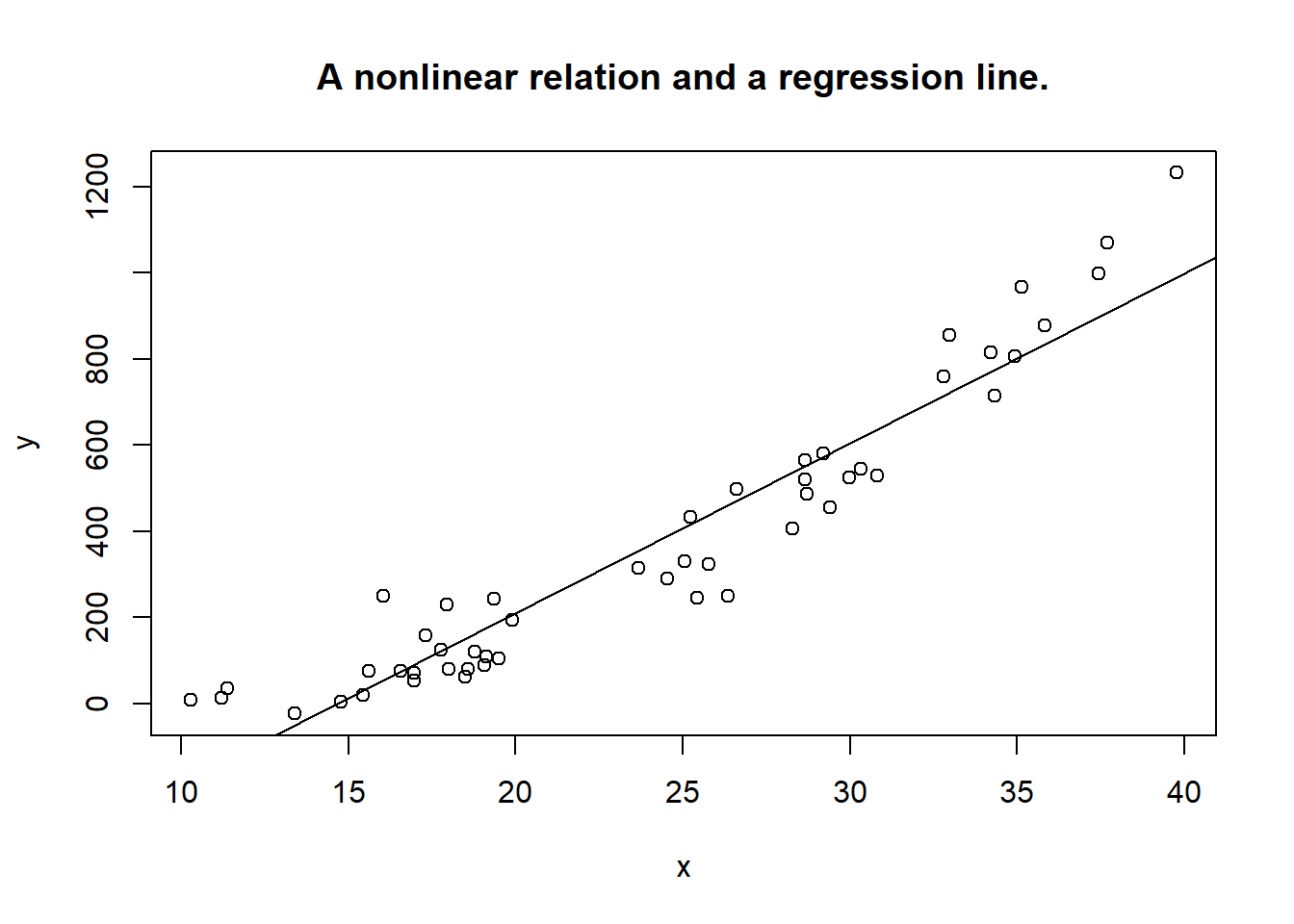
Figure 5.4: Nonlinear relation.
5.7 Diagnostic plots for the regression object.
R offers a plot function that produces four “diagnostic” plots that can be used to detect problems regarding a regression analysis.
We will just briefly look at what they can be used for here, without going in much detail. We can continue with our running example with the Duration vs Distance data. The code is simply as follows
The code par(mfrow = c(2,2)) tells R to make all four plots in one go.
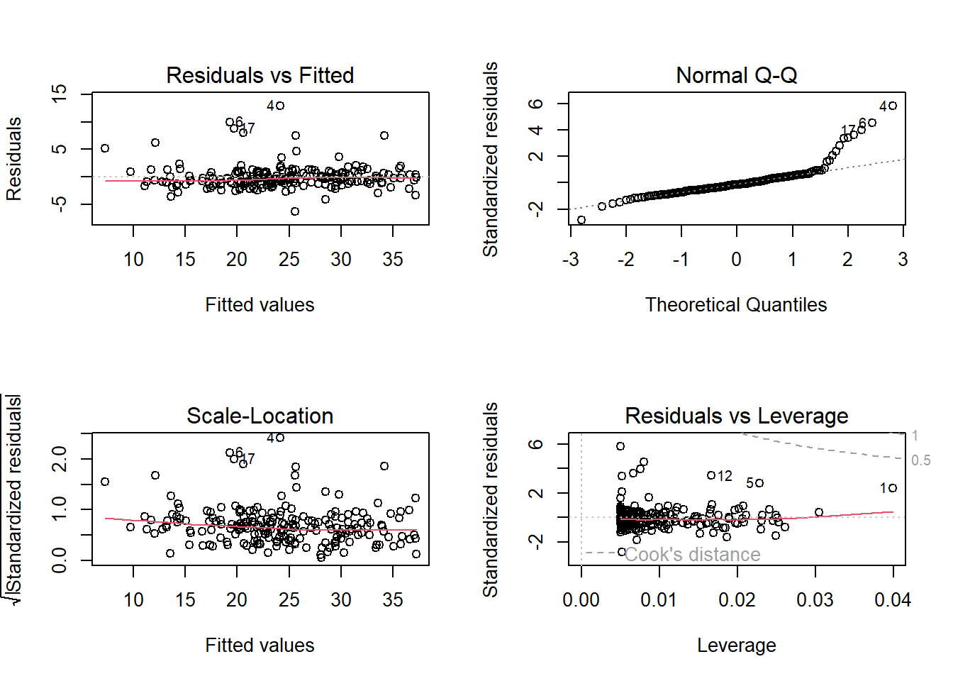
The first plot “Residuals vs Fitted” shows residuals \(e_i\) versus the predicted values \(\hat{y}_i\). This plot should ideally show points nicely spread horisontally with the red line flat. It is used mainly to assert that the data fits to a linear model.
The “Normal Q-Q plot is a normal plot of the residuals. Since we assume that the error term is normally distributed, we should ideally have our points along a straight line here. In the example, it looks like there are some problems in the upper range there.
The “Scale-Location” plot can be used to detect violations of assumption D, so any pattern different from a flat spread of the points could be a signal that this assumption is troublesome.
Finally the “Residuals vs Leverage” plot is mainly used to detect so-called influential outliers. These are single observations with a relatively large distance to the mean in the \(x\)-dimension (leverage) plus a relatively large residual. So points in the upper or lower right corner are considered troublemakers.
Regarding the example we look at here, the most problematic assumption is probably about the normality of the error term. It is typically a topic of a more advanced course in regression to go deeper into such problems of regression models. We should however be aware of the risk of drawing invalid conclusions when some key assumptions are violated.
This chapter has introduced basic linear regression models as a tool for analyzing relations between variables. We have discussed how to interpret the general model. We learned about the distinction between the theoretical model and the estimated model. Certain assumptions need to be satisfied in order to get reliable results from regression analysis. These were discussed. We saw specifically how the parameter estimates comes from the least squares method. We seek the linear model that minimizes the square sum of the residuals.
We have seen that regression analysis can be easily done with R. The user (you) must take responsibility for checking basic assumptions, as R will just obey your commands, whether good or bad. We have gone through the R regression object and some of its content, and you should be able to explain almost all of it by now. There are coefficient estimates, confidence intervals for \(\beta_i\), there are some \(t\) values, and some P-values. We saw the splitting of variation, the square sums \(SSE\) and so on. Remember \(R^2\)? And \(S_e\)? They both tell us about the estimated model’s prediction accuracy. We discussed how basic model assumptions can be checked with R. You will acquire familiarity and hopefully some good feelings about regression analysis through the practice offered with the exercises related to this section. Our next big step forward will be to allow models with several \(X\) variables. Such models can look like \[ Y = \beta_0 + \beta_1 X_1 + \beta_2 X_2 + \beta_3 X_3 + \mathcal{E} \;,\] in case of three \(X\) variables. If you understand most of this current chapter, you will have no problem moving there.
5.8 The stargazer package
We end this chapter with a nice utility package in R. It is the package stargazer which is specifically designed to produce nice(r) tables from a regression analysis. It will be particularly useful in later chapters, when we compare different models on the same data. Let us now just look at the basic look for two-variable regressions. We proceed with our Distance/Duration model. We created a regression object regfit, and we saw how to inspect it using e.g. summary. We can also do as follows
##
## ===============================================
##                         Dependent variable:
##                     ---------------------------
##                              Duration
## -----------------------------------------------
## Distance                     2.226***
##                               (0.054)
##
## Constant                      1.162**
##                               (0.584)
##
## -----------------------------------------------
## Observations                    200
## R2                             0.895
## Adjusted R2                    0.895
## Residual Std. Error      2.218 (df = 198)
## F Statistic         1,691.353*** (df = 1; 198)
## ===============================================
## Note:               *p<0.1; **p<0.05; ***p<0.01
This follows the traditional way of presenting regression results, with coefficient estimates and their standard deviations in (…). In addition, we get a more limited summary of the regression. There are lots of parameters to this function, just as an example we can replace the standard deviations with confidence intervals as follows.
##
## ===============================================
##                         Dependent variable:
##                     ---------------------------
##                              Duration
## -----------------------------------------------
## Distance                     2.226***
##                           (2.120, 2.332)
##
## Constant                      1.162**
##                           (0.017, 2.307)
##
## -----------------------------------------------
## Observations                    200
## R2                             0.895
## Adjusted R2                    0.895
## Residual Std. Error      2.218 (df = 198)
## F Statistic         1,691.353*** (df = 1; 198)
## ===============================================
## Note:               *p<0.1; **p<0.05; ***p<0.01
Of course, to be able to use this we need to run install.packages(“stargazer”) in Rstudio once.