Chapter 3 A brief intro to R and Rstudio
3.1 Introduction
We have chosen to use R/Rstudio as our data analysis tool in Log 708. In pace with the ever increasing interest and use of data analysis in science and business, R is becoming one of the most popular tools and by now has a huge numberof active users. Some of the advantages of using R/Rstudio is:
- It is free, so there is no need for expensive licenses
- You can install it on your own PC, so there is no dependency on resources from school or workplace.
- The huge and friendly user base makes almost any problem solveable through google search
- It is fundamentally code based, so it enhances reproducible research/work
- It contains numerous different packages which makes it useful in almost any data analysis task we might imagine. (E.g. visualization, machine learning…)
- It is platform independent, so should work similarly on PC, mac, etc…
We will soon realize that R/Rstudio is a HUGE system with multiple different uses. One that is maybe less known is to use R as a tool for writing scientific documents. In fact the compendium you are now reading is entirely written in R with the use of packages to facilitate e-book and pdf versions.
In Log 708 we shall only touch the very basics of this system, and focus on what we need for relatively simple statistical analyses.
In the canvas room for Log 708, there will be video clips available that shows many of the same things that are presented here. You will also find numerous clips on YouTube and other online sources of information on the basics.
3.2 Installation
The first thing we need to do is to actually install R and Rstudio on our computer. If you do not already have a working installation we strongly recommend that you watch the video about installation that you will find in Canvas. Note that you need to install R first, then Rstudio.
You can go to the link below, then find the link to R installation, and then install Rstudio.
https://www.rstudio.com/products/rstudio/download/#download
Some tips:
Note that the installation of R may require that you choose a particular version suitable for your PC, for example the Windows versions of R are either 32 bit or 64 bit. Practically all PC’s that are less than 10 years old will run 64 bit. If you have an old PC, you can check on Windows by going to “Settings” choose “System” and then “About” to see what Windows version you have, and what processor you run on. Similarly there may be a choice of versions for Mac-OS, with similar ways to check your system specifications.
If you are asked to name file locations during installation, avoid using files or folders with letters not in the English alphabet, e.g. the Norwegian “æ, ø, å”. Numbers are OK, so “Rstudio-2023” should work, while “OneDrive-Høgskolen-i-Molde” may cause trouble.
The Rstudio system is now part of a wider software system called “Posit”. That may cause some of our web searches about Rstudio to also contain information about Posit, but this should not cause any problems.
If for some reason you can not make the installation work, there are several other ways we can use R/Rstudio in this course. Detailed information about such options will be given in the course material on our learning platform (Canvas) and in lectures.
The other videos in the R introduction series on Canvas gives a visual overview of the system, which is difficult to reproduce here, so we focus here on other details relevant to the course.
3.3 Rstudio window frames
Rstudio has four window frames, console, editor, environment, files and figures
- Console: Here we do the interactive work, testing things, doing quick calculations etc.
- Editor: Here we edit our source code files.
- Environment: Here we can overview and inspect the data that we have in work.
- Files and Figures: Here we can overview our working directory, and we get figures out here.
To learn more about these different parts, consult video clips on Canvas.
3.4 About using R in these notes.
In the following you will see a lot of R code, looking like this:
## [1] 1 2 3Don’t worry if you do not understand the code by now, we will explain below.
The first block here has two lines of code. When we run this code, the output is the vector (1, 2, 3). The part of code that is preceded by # are comments, these are ment to explain to the creator and other readers of the code what was intended.
The output in these notes is usually preceded by ##. Note that if you read this online, you can copy the code and paste it into your R console (or editor). Clickc the icon in the upper right corner to copy a whole block.
If you edit a code file which we call an “R script”, it will look as in the upper block here. You will save your script as “filename.R” on your disk, and once you have made a working script file, you will have it for the rest of your life! (This is one of the TRUE HUGE benefits of using a system like R. You will always be able to go back and reproduce EXACTLY what you did half a year or more ago.)
3.5 Rscripts
In this course we will mainly do our R work by using R scripts. These are just ordinary text files, which contains
lines of R code and comments as we have seen above. To open a new R script, you should go to the “File” menu, choose “new
file” and “R script”. you will see the file as “untitled” in your editor part of R studio.
You can then save the file with a name, e.g. “myfirstscript.R”. You see that R scripts always have
the suffix .R in their name. There are several different ways to use R scripts, one can for example run a whole file at once to execute a certain sequence of codes. More often we can use an R script to hold several more or less related
codes, and then execute selected parts of the code. On windows, put the cursor at some line of code, then press ctrl + ENTER and the code will run in your console. If you have successfully installed R and Rstudio, it is a good idea to start Rstudio now, open a new script file and proceed to go through the examples below, by copying and pasting the code examples into your R script, and executing part by part as suggested above.
3.6 Getting started
The first fundamental thing to understand is that R and Rstudio are not the same thing. We can think of Rstudio as an advanced interface to R, while R is the underlying “engine” that does most of the real work for us. The whole menu system that you see in Rstudio can be used to control parts the engine, but more often we will use code that is managed in Rstudio to give orders to R.
The second fundamental thing to understand is that R is a programming language. This essentially means we communicate with R through (sequences of) written statements, i.e. code. This code can be anything from very simple to extremely complicated, in this course we will stay safely on the simple side.
There is one and only one way to learn to use R and that is to start using R.
3.6.1 Vectors
It is important to understand that when you work with R we are constantly using objects. The fundamental object type in R is a vector. A vector then, is simply a numbered series of numbers, words (and some other types). the rule is that all elements in a vector must be the same type, i.e. all numbers or all letters and so on.
Before looking at some vectors we must introduce the function c(...).
This function is fundamental to R, what is does is basically to take anything you give to it and (if possible) pack it into a vector. Secondly we must underline the assignment operator: This is the sign <-. If we write
a <- 2 it means: “make the object a and assign the value 2 to it. So whenever we refer to a later it will have the value 2. (Unless changed by other code.)
So, let us look at some vectors. Remember # ... means a comment, that is not part of code.
#make a vectors (3, 2, 1) and (4, 5, 6)
x <- c(3, 2, 1)
y <- c(4, 5, 6)

#add together and print result
x + y
## [1] 7 7 7So as expected we get the result (7, 7, 7). Note that we did not save the result x + y in another object, so the result is “lost”. If for some reason we wanted to keep it we should have done this
## [1] 7 7 7This code assigns the value of x + y to a new object called z, then outputs z. We should note that most operations in R are vectorized, which means the operation is applied to each component of the vector. Suppose we want to have all the squares of x, we simply write
## [1] 9 4 1The result is as expected.
3.6.1.1 Accessing elements of vectors.
Suppose we want only the third element of x above, then we use simple “indexing” so we write
## [1] 1R vectors can contain other types than numbers. Notably are “character” and “logical” vectors. A few examples will show this. Try this and look at the results:
Here cities is a character vector, test is a logical vector with values TRUE and FALSE.
3.6.2 Functions
The second fundamental building block of R is the concept of a function. We will for now only consider built-in function, it is however simple to design your own functions - which you will do once you get to a slighly more advanced level. We can look at some very basic functions now (there are thousands available…)
## [1] 3## [1] 6## [1] 2## Min. 1st Qu. Median Mean 3rd Qu. Max.
## 1.0 1.5 2.0 2.0 2.5 3.03.6.3 Mistakes and errors
Starting to write R code means you are going to make mistakes and get error messages. This happens every day even for trained R users, so don’t be put off by this. If you can’t figure out where your error lies, try to search the web, ask a fellow student or one of the teachers involved in the course. A very common source of error is when we try to do something with the “wrong” type of data. For example, if we accidentally try to sum the variable cities defined above, we get trouble as there is no defined way in R for adding character strings. This kind of error is something every R user runs into from time to time.
Trying this should give something like
A handy function here is the str function (short for “structure”) which tells what the type of our objects are,
so we can try
## num [1:3] 3 2 1## chr [1:3] "Molde" "Kristiansund" "Alesund"That shows x is an numerical vector, while cities is a character vector.
3.6.4 Probability distributions.
R has built-in almost every known probability distribution, (google “R probability distribution” to learn more).
let’s look at some fundamental ones. Starting with the normal distribution(s), we have functions
dnorm, pnorm, qnorm and rnorm these are respectively the probability density, the cumulative distribution the inverse cumulative distribution and a random generator function. So if \(Z\) is a standard normal variable, what is the probability \(P[Z \leq 2]\)? We get this by writing
## [1] 0.9772499We can write ?pnorm to get into R’s help system for the function pnorm (or you can go through help via Rstudio). Here we learn (i) that pnorm is a more general function, we can add the arguments mean and sd to the function call to find probabilities for general normal distributions. In addition, the function is vectorized, so we can give a vector of values for which we want to compute probabilities. Suppose the demand for icecream on a day is \(X\), a normally distributed variable with mean 200 and standard deviation 40, what is the probability that \(X \leq 200, 250, 300\)? We learned how to do this via standardization and using a normal table in chapter 2.3. Now
let’s ask R:
#define vector of possible values
V <- c(200, 250, 300)

#calculate the three asked-for probabilities:
P <- pnorm(V, mean = 200, sd = 40)
#look at P:
P
## [1] 0.5000000 0.8943502 0.9937903This code also illustrates a nice R feature, where the function pnorm has a “default” behaviour when called as pnorm(2) and then a more general behaviour when we specify additional parameters. This is very common with R functions, so that one single function can allow for very flexible usage.
3.6.5 Sequences
We sometimes want to make structured sequences of numbers in R. Try the following and see what you get:
One common use of this is to select out a subset of a vector: The code below shows how to draw randomly 12 numbers from a normal distribution, then select the first 8.
##  [1] 34.38975 30.56318 33.06607 28.22450 29.66340 27.22514 32.25991 29.66217
## [9] 29.80773 30.69983 26.59025 32.56449## [1] 34.38975 30.56318 33.06607 28.22450 29.66340 27.22514 32.25991 29.662173.6.6 Data Frames
Now we have played a little bit with the basic vector object in R. The next step is to look at what we call data frames. These corresponds nicely to what we call a “data set”, but it should be understood that a data frame is an internal data object in R, different from a data file which we shall look at later on. We can only say at this point that when we read a data file into R, the data will always be stored in a data frame. So what is a data frame? Let us first make a very simple data frame. We will call it “DF”, which is a common name to use when we play with small examples. (In general a dataframe can have any name you like.)
#create example data
DF <- data.frame(name = c("Jim", "Jane", "Tim", "Bill", "Joe", "Mary", "Fred"),
                 height = c(183, 178, 189, 175, 179, 169, 183),
                 weight = c(80, 73, 82, 75, 73, 64, 81))

#look at it
DF
## name height weight
## 1 Jim 183 80
## 2 Jane 178 73
## 3 Tim 189 82
## 4 Bill 175 75
## 5 Joe 179 73
## 6 Mary 169 64
## 7 Fred 183 81So, we see that the data frame DF correspond to what we usually think of as a data set: A collection of columns of the same length and with the same type of data within each column. However the data types can be different in different columns, as we see. In fact, a data frame is simply a list of vectors of identical length, with individual names. In general data frames can have a large number of columns (also called variables) and a HUGE number of rows.
So for starters, let’s see how we count rows and columns, and also how to find the variable names in a data frame.
## [1] 7## [1] 3## [1] "name" "height" "weight"Very handy when we work with dataframes are the functions head and tail. They allow us to show the first and last few rows of a dataframe. The default number is 6, so if we write head(DF) we get the first 6 rows. We can also try
##   name height weight
## 1  Jim    183     80
## 2 Jane    178     73
## 3  Tim    189     82
## 4 Bill    175     75
And you can try tail(DF, 5). This is useful when we have a big dataframe, but only want to check the look of it with a few rows.
3.6.6.1 Accessing columns
Sometimes we want to access a single column, say the height column from DF. This is a vector of numbers, and we get it by writing DF$height, for example we can compute the mean and standard deviation as follows:
## [1] 179.428571 6.4253963.6.6.2 Subsetting
It is quite common that we want to extract a subset of a data set for analysis. Often this is in terms of a logical condition on one or more variables. This can be done in different ways in R, one is to use the subset function.
This works on data frames and returns data frames. Let us get the following subsets from DF:
- A = all persons taller than 175cm
- B = all persons taller than 175cm and weighting less than 80 kg
##   name height weight
## 1  Jim    183     80
## 2 Jane    178     73
## 3  Tim    189     82
## 5  Joe    179     73
## 7 Fred 183 81## name height weight
## 2 Jane 178 73
## 5 Joe 179 73You will also commonly see indexing methods used to access parts of a data frame. Basically, using DF as an example, we can write DF[2, 3] to access the particular value in row 2, column 3 of DF it is however not usual that we need to do such things for basic statistical analysis. What is more common is to want to select say the first 4 rows, or the last two columns of a data frame. Then we can do
##   name height weight
## 1  Jim    183     80
## 2 Jane    178     73
## 3  Tim    189     82
## 4 Bill 175 75## height weight
## 1 183 80
## 2 178 73
## 3 189 82
## 4 175 75
## 5 179 73
## 6 169 64
## 7 183 81As an intelligent reader, you realize that DF[1:4, ] gives the same as head(DF, 4).
It can be helpful to realize that DF[1:4, ] is a new dataframe, so we can do this:
##   name height weight
## 1  Jim    183     80
## 2 Jane    178     73
## 3  Tim    189     82
## 4 Bill    175     75
The View function will show a data frame in “spreadsheet” view, which is sometimes a better way to look at data.
3.6.6.3 Visualization
One of the reasons for the widespread popularity of R, is the extremely rich possibilities for visualization of data. We can not go into any detail of this here, but we note that it is all based on data frames, which we are now learning about. A very basic visual display of DF is to show the relationship between height and weight. Using “base R” plotting we can do like this
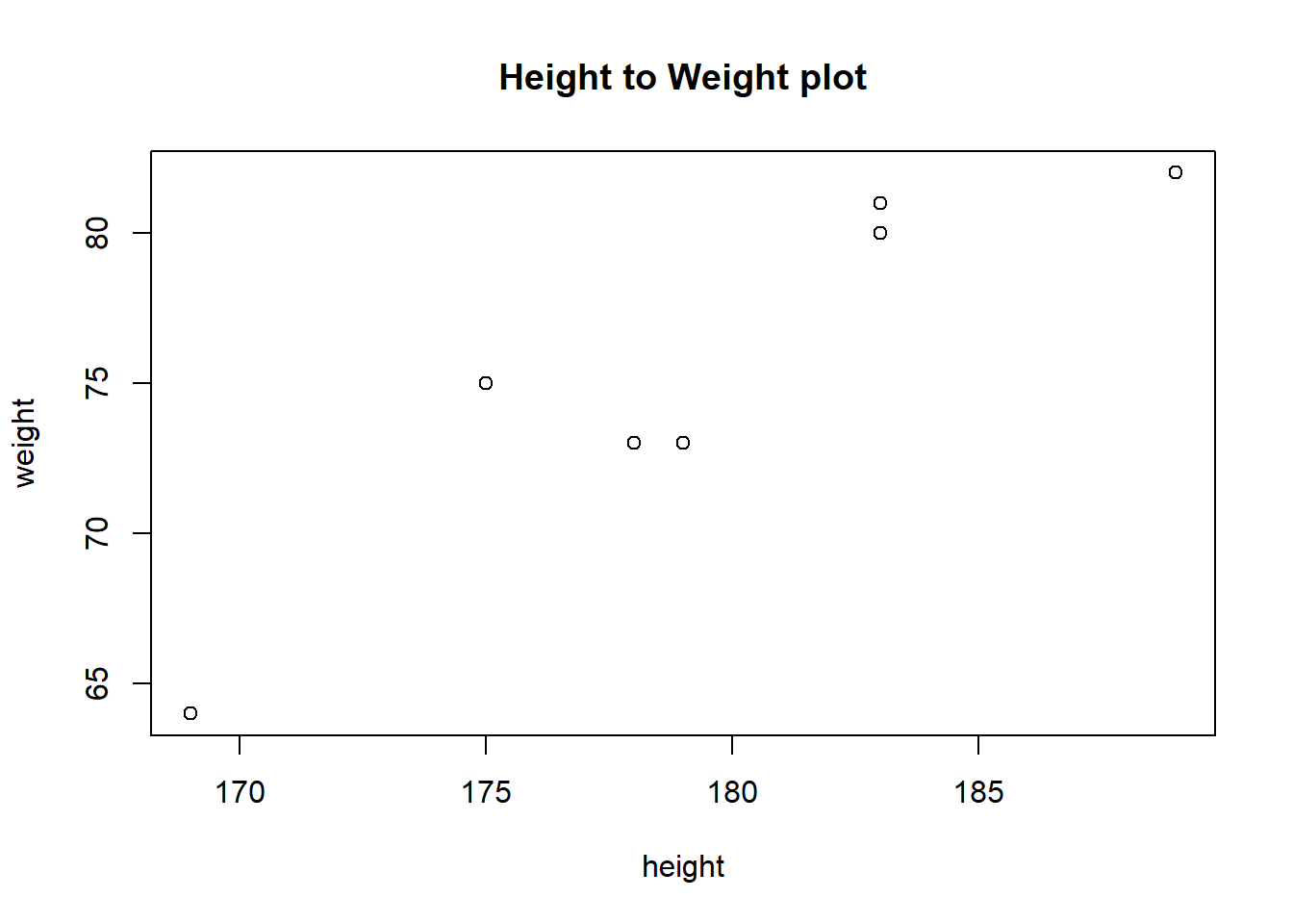
Here we used the with function to say that we want to plot with variables taken from the DF data frame.
An equivalent code is the following, which to use is a matter of taste. main is a parameter to the plot function, assigning the title of the plot.
The plot function has a large number of parameters that can be adjusted to change the appearance of a plot. From Rstudio we can save a plot to disk or copy-and-paste into a document.
A few more examples. We already saw the dnorm function representing the normal density. Let us make a plot of the this function in the standard case \(\mu = 0, \sigma = 1\). We show two ways, (i) build data with one vector for \(x\) values, one with \(f(x)\) values and use this as data for the plot. (ii) use the built-in function curve to plot directly.
Using plot:
#generate x-values
x <- seq(from = -4, to =  4, by = 0.1)
#compute normal density from x
fx <- dnorm(x)

#look at the first 10 values
head(data.frame(x, fx), 10)
## x fx
## 1 -4.0 0.0001338302
## 2 -3.9 0.0001986555
## 3 -3.8 0.0002919469
## 4 -3.7 0.0004247803
## 5 -3.6 0.0006119019
## 6 -3.5 0.0008726827
## 7 -3.4 0.0012322192
## 8 -3.3 0.0017225689
## 9 -3.2 0.0023840882
## 10 -3.1 0.0032668191#make plot
plot(x, fx,
main = "Standard normal density",
ylab = "f(x)",
type = "l",
lwd = 2)
#add horisontal line at y = 0:
abline(h=0)
The parameters to the plot function here is main, specifying the title for the plot, ylab sets the label for the \(y\) axis, type = "l" sets what type of plot we want (“l” for “line), and lwd specifies the line width.
In the code here, we write the sequence of parameters (i.e. main, ylab, type...) on separate lines. This is just to make the code easier to read, we could equally well have written
The choice is really a matter of taste. Now let us see option (ii) for making the same plot. This utilizes the fact that dnorm is already an existing function. So it is more compact, like this:
curve(dnorm(x),
      xlim = c(-4, 4),
      main = "Standard normal density",
      ylab = "f(x)",
      type = "l",
      lwd = 2)

abline(h=0)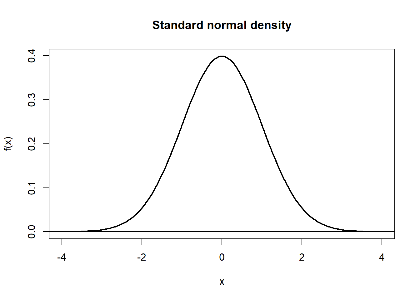
So far we are using base R plotting. The real power of R as a visualization tool is unleashed with the package ggplot2 which you can easily learn about at a later stage. As is typical with R you can find almost any kind of example on the web, along with the exact code that generated the picture. See e.g.
https://www.r-graph-gallery.com/.
##   Sepal.Length Sepal.Width Petal.Length Petal.Width Species
## 1          5.1         3.5          1.4         0.2  setosa
## 2          4.9         3.0          1.4         0.2  setosa
## 3          4.7         3.2          1.3         0.2  setosa
## 4          4.6         3.1          1.5         0.2  setosa
## 5          5.0         3.6          1.4         0.2  setosa
## 6          5.4         3.9          1.7         0.4  setosa
# A basic scatterplot with color depending on Species
ggplot(iris, aes(x=Sepal.Length, y=Sepal.Width, color=Species)) +
geom_point(size=3) +
geom_smooth(method = lm, se = FALSE)## `geom_smooth()` using formula = 'y ~ x'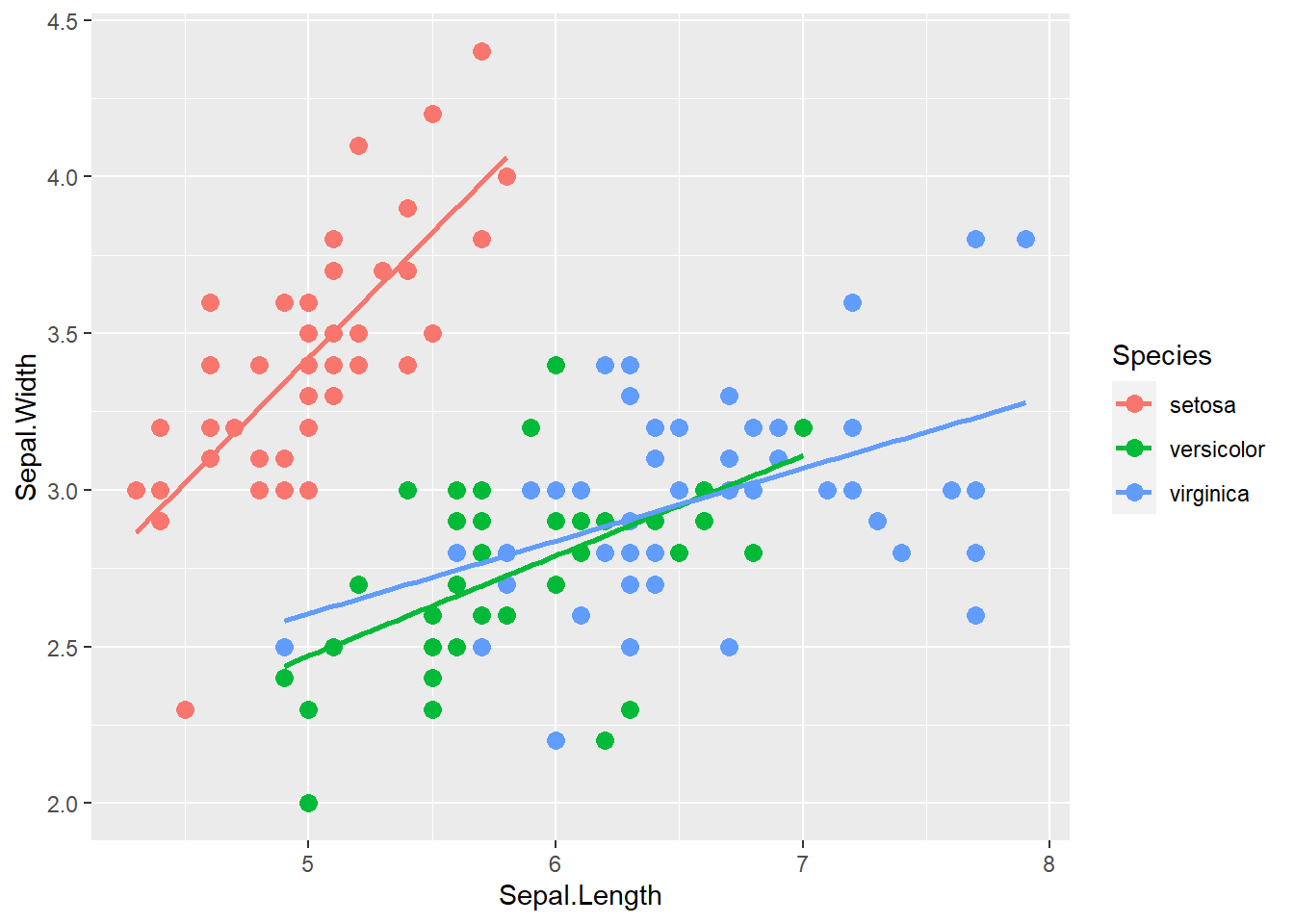
3.6.7 NA
In our data sets, we sometimes encounter missing data, so for some reason a value is not recorded as it should be.
In R such missing values are labelled as NA meaning Not Available. We should always watch out for this, because some functions will not by default compute a result if a vector is having NA values. If so, we can use the na.rm option to force the calculation to be processed. Let’s see an example.
## [1] NAThe result is NA, so R will not give a value for the mean, because there is an NA there. To force a calculation using the existing values, we go like this.
## [1] 6.7142863.6.8 Factors
R factors is a concept that is sometimes difficult to get around, you should try to understand the following, but not be put off if you don’t.
A categorical variable in data is a variable that only can have one of a limited set of values. For example suppose that our friends in the data frame DF were students in a course, and we found their grades to be A, B, B, D, D, B, D. We can extend the data frame with the grades as follows.
##   name height weight grade
## 1  Jim    183     80     A
## 2 Jane    178     73     B
## 3  Tim    189     82     B
## 4 Bill    175     75     D
## 5  Joe    179     73     D
## 6 Mary    169     64     B
## 7 Fred    183     81     D
Now, this looks fine - but there is a thing missing here. If we now ask R to count the grades, e.g. to show the distribution of grades it will only count A’s, B’s and D’s. We use the table function as follows.
##
## A B D
## 1 3 3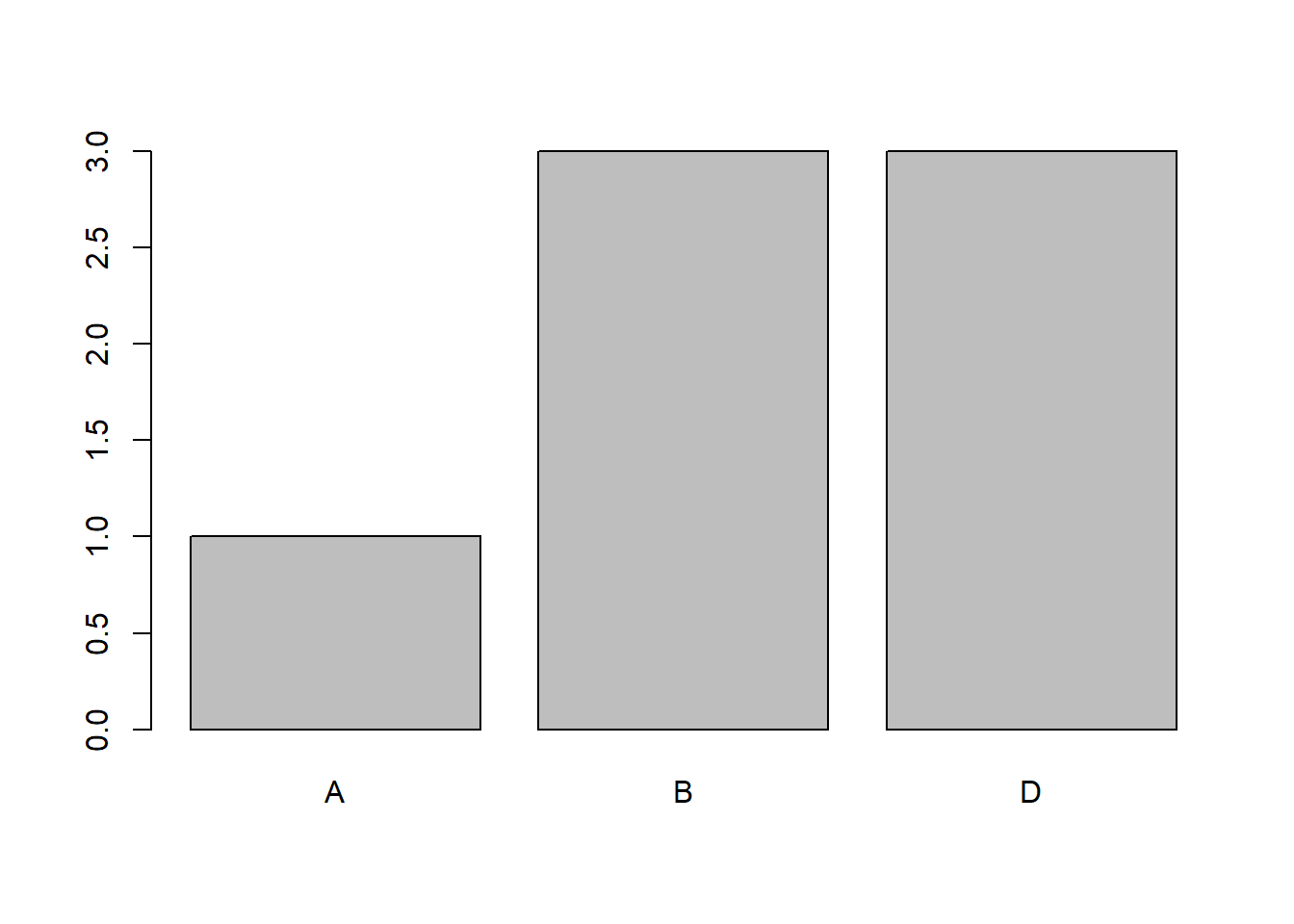
So, correctly - there are 1 A, and so on. What is missing is that we might want to count 0 C’s, E’s and F’s also.
Here is (one place) where we need to make grade an R factor. Basically, we give it something called levels whichs are all the values it could possibly take. So grade is still a character vector, but with an added property: the levels.
So look at this.
#add column grade as a factor:

DF$grade <- factor(c("A", "B", "B", "D", "D", "B", "D"),
                   levels = c("A", "B", "C", "D", "E", "F"))

DF
## name height weight grade
## 1 Jim 183 80 A
## 2 Jane 178 73 B
## 3 Tim 189 82 B
## 4 Bill 175 75 D
## 5 Joe 179 73 D
## 6 Mary 169 64 B
## 7 Fred 183 81 DIt looks pretty much the same, but see what happens when we do the count using table:
##
## A B C D E F
## 1 3 0 3 0 0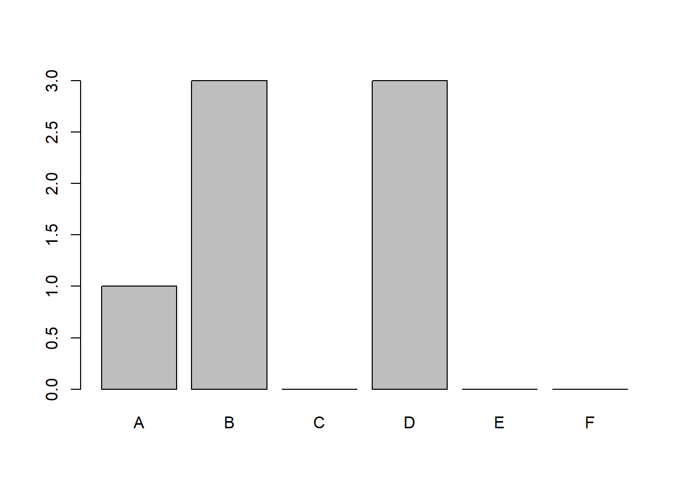
The difference here is one motivation for wanting to use R factors for categorical data. We will come back to this concept later on, for now - hopefully this was understandable.
3.6.9 Sampling
Random sampling can be a useful method when it comes to learning R and statistics. It basically means we ask R to perform a draw of some sorts for us. R utilizes a random generator to do this, and this should preferably be started with a statement in your code of the form set.seed(51351). This ensures that your random sequence can be reproduced, which can be important if you get trouble with your code. The number 51351 is totally arbitrary. Use whatever.
We look at two variants of sampling here.
3.6.9.1 Sampling from a probability distribution.
We have seen that R has built in probability distributions. For simplicity let’s stay with the normal. Let’s make two samples of 100 \(N(30, 10)\) variables, and look at their histograms.
#initialize random generator
set.seed(12342)

#draw samples
normals <- data.frame(x = rnorm(100, 30, 10), y = rnorm(100, 30, 10))

#allow side-by-side plots
par(mfrow=c(1, 2))

#make histograms
hist(normals$x, main = "Histogram of x", xlab = "x")
hist(normals$y, main = "Histogram of y", xlab = "y")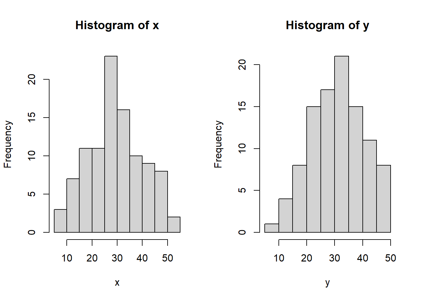
We know that we use the sample means \(\bar{x}, \bar{y}\) as estimates for the true mean \(\mu\). In the sampling above we know that \(\mu = 30\), so it can be interesting to see how close are the sample means.
## [1] 29.36899 31.15871We see as expected, the sample means are close but not equal to 30.
3.6.9.2 Sampling from a vector or a dataframe
We will look at the sample function. Basically this allows us to draw n times from a given vector x.
There is a logical parameter replace so if this is TRUE we draw with replacement (i.e we don’t remove drawn objects
from the vector after each draw.) Some examples.
## [1] 3 4 6 20 14 17 4 16 12 4## [1] 10 19 15 16 7 2 5 18 11 12See the difference? Now: How would you simulate 30 tosses of a die? And show the count of each value 1, … ,6? Think a bit before you look at the code below.
#define possible outcomes
v <- 1:6
#sample 30 times with replacement
S <- sample(v, 30, replace = TRUE)
#count usiung "table" function
counts <- table(S)
#show results
counts
## S
## 1 2 3 4 5 6
## 4 3 7 4 2 10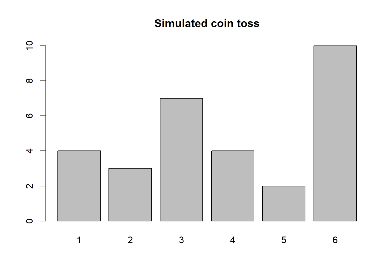 Sometimes we might want to sample rows from a dataframe. There are R packages (see section 3.10.1 below about packages) that does advanced such sampling for us. Here, let’s just see a basic approach using
 base R. What we do is to sample a vector of row numbers, then extract the corresponding rows. We can use our small data frame DF as example, even though the typical use of this method is to sample say 1000 rows from a HUGE dataframe with maybe 10 million rows, to do some initial experiments for example. The beauty is that the code is the same. Say we want to sample k = 4 of the n = 7 rows. We show the general method.
#set k
k <- 4
#count rows in DF
n <- nrow(DF)
#sample some rows from the vector 1:n, with no replacement.
S <- sample(1:n, k, replace = FALSE)
#Extract the rows in DF corresponding to S.
DF[S, ]
## name height weight grade
## 5 Joe 179 73 D
## 6 Mary 169 64 B
## 4 Bill 175 75 D
## 7 Fred 183 81 DIf you want the result sorted, use this
##   name height weight grade
## 4 Bill    175     75     D
## 5  Joe    179     73     D
## 6 Mary    169     64     B
## 7 Fred    183     81     D
3.7 The working directory and file paths
Before going further we need to address an important concept when working with R, the working directory. When you run an R session, you are always working in some particular directory (a folder) on your computer. You can find your working directory path by this code
## [1] "M:/Undervisning/AppStat Kompendium/Rbook2024/Log708Compendium"The output here is specific for the particular session that the author was running when writing this compendium, you will of course get something else on your machine. On a Mac this may look a little different, but in principle it should be the same structure. The character string above shows the path from the “M” disk down to the actual directory, so there are several folders in between. To change the working directory, use the function setwd() e.g. as follows
The Rstudio editor does a bit of “autocomplete” operations, so if you write say setwd("M:/ and hit “TAB” it will usually be able to list the possible alternatives of subfolders to "M:/" or whatever you start with. Try this. Now.
Sometimes you want to move up or down one or two steps in the folder hierarchy defined in the path. Then you can use a few shortcuts to save some writing:
#move to folder above:
setwd("..")
#move two folders up:
setwd("../..")
#move to subfolder "X" of the current working directory
setwd("./X")
To see all the files and folders in the working directory, use dir().
3.8 Data files
Data files are where we store and find our data when finishing/starting an R session where we want to work with data. R can import data in different formats, for example excel files or SPSS files. Most often for R we want to have the files in “comma-separated” form, which means the data file is just a text file where each row of data is a row in the file, and each value in a row is separated by a “,” (or a “;”). Such datafiles have the suffix `.csv”
In Rstudio you can open (read) data files using the File/Import Dataset menu. Note that you will get the corresponding code as a “bonus”, and after some time you can learn by this how to directly write the code that reads a file. It is always good to have everything written in code in an R script, also the “read file” part. It can look as follows where this is starting from the working directory shown above. Let’s see.
## [1] "M:/Undervisning/AppStat Kompendium/Rbook2024/Log708Compendium"What’s in this folder?
##  [1] "__output.yml"            "_book"
##  [3] "_bookdown.yml"           "_bookdown_files"
##  [5] "_output.yml"             "01-intro.Rmd"
##  [7] "01-intro_fckd.Rmd"       "02-random_vars.Rmd"
##  [9] "02-random_vars_files"    "03-Rintro.Rmd"
## [11] "04-testing.Rmd"          "05-basic_regression.Rmd"
## [13] "06-multreg.Rmd"          "07-nonlinreg.Rmd"
## [15] "08-logtrans.Rmd"         "10-references.Rmd"
## [17] "book.bib"                "Data"
## [19] "Figures"                 "index.Rmd"
## [21] "Log708Compendium.Rmd"    "Log708Compendium.Rproj"
## [23] "Log708Compendium.toc"    "Log708Compendium_files"
## [25] "obsolete"                "packages.bib"
## [27] "preamble.tex"            "README.md"
## [29] "rsconnect"               "style.css"
## [31] "tikz1e60768223d4.log"    "tikz2bc42be21fc.log"
## [33] "tikz3102801e71.log"      "tikz314033e572ef.log"
## [35] "tikz47ecdae5192.log"     "tikz782219c1a.log"
## [37] "tikzd1014397630.log"
There is a lot of stuff, but I have the “Data” folder, let’s check that out:
##  [1] "AirBnBSing2.csv"          "alkfos.csv"
##  [3] "clock_auction.csv"        "Company_sales.csv"
##  [5] "Cruiseship.csv"           "Cruiseship4.csv"
##  [7] "desktop.ini"              "flat_prices.csv"
##  [9] "flat_prices.sav"          "flat_prices_1.sav"
## [11] "flat_prices_extended.sav" "Hospital-durations.sav"
## [13] "Hospital_durations.csv"   "HotelAS.csv"
## [15] "meat_brands.csv"          "meat_brands.sav"
## [17] "MetalAS.csv"              "Money-vs-time.sav"
## [19] "Money_vs_time.csv"        "Mt.csv"
## [21] "newdata.csv"              "Norfirms.csv"
## [23] "Nycflights2.csv"          "R-square-examples.sav"
## [25] "Tdur.csv"                 "TeleAS.csv"
## [27] "Trip_durations.csv"       "Trip_durations.sav"
## [29] "used_cars.csv"            "Wages.csv"
## [31] "Wages.sav"                "WaterWorld.csv"
## [33] "WaterWorld.sav"           "world95.csv"
## [35] "world95_mod.sav"
These are all data files, I want the “flat_prices.csv” file into a data frame, so I go
##   price area rooms standard situated town distcen age rent
## 1  1031  100     3        2        6    1       5  15 2051
## 2  1129  116     3        1        5    1       4  42 2834
## 3  1123  110     3        2        5    1       3  25 2468
## 4   607   59     2        3        5    1       6  25 1940
## 5   858   72     2        3        4    1       1  17 1611
## 6   679   64     2        2        3    1       3  17 2039
So, now we have taken the data from a disk location, to a dataframe in our R session, and we can do whatever we want with it. Note that the data in this cases was separated by “,” so we used read.csv. In case the data are separated by “;” there is a corresponding function read.csv2.
The data here are flat prices for a number of sold flats in three towns (Kristiansund, Molde, Ålesund)
For example we can use a function tapply from base R to summarize the prices that are recorded in the three towns.
## $`1`
##    Min. 1st Qu.  Median    Mean 3rd Qu.    Max.
##     607     847    1031    1008    1177    1625
##
## $`2`
##    Min. 1st Qu.  Median    Mean 3rd Qu.    Max.
##   423.0   737.5   931.0   949.5  1072.2  1866.0
##
## $`3`
##    Min. 1st Qu.  Median    Mean 3rd Qu.    Max.
##   556.0   849.5  1026.0  1064.5  1302.5  1698.0
We see some differences in the mean prices. We can make a boxplot for prices in each town as follows,
#make boxplot for each town.
with(flatprices, boxplot(price ~ town, main = "Price distribution in the towns."))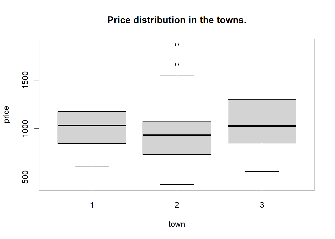
Here, the construction price ~ town means “price depending on town”, so we want the plot to be for each category of town. This is called an R formula and we will use it a lot later on.
We will look more closely at these data later, for now the main point is to work with data files. Suppose we do some work on the data, e.g. calculate a column of square meter prices. Then we want to quit working, and we want to save the data to disk with name “newdata.csv”. We can then use the base function write.csv for this purpose. It goes like this:
So, next time you want to work with these data you can use
For training purposes base R comes with a number of datasets which we may use in some examples. Try data() to get a list of available data. In addition many R packages comes with their own data sets. For example the base package (which is always active) contains a dataset called mtcars. Write data(mtcars) to get a dataframe with these data.
When you exit from an R session you will usually get a question like
Save workspace image to M:/Undervisning/AppStat Kompendium/Rbook2021/Log708Compendium/.RData? [y/n]:
In this case, R asks whether you want to save all the dataframes, vectors, and so on (i.e. all objects) in your working session into a special type of file, called “.Rdata”. When you start R again it will load all of the objects into your “environment” (See below) so you can continue work. This is OK if you are just leaving for a short break, or want to continue next day. For any longer time of saving it is recommended that you save data in ordinary data files, and the code that produces relevant objects in script files. (The problem with .Rdata files is that there is no documentation of how things were calculated, so often it can be difficult to know what you actually have.)
3.9 Online access to course data files.
It is really important that (over time) you learn how to read and write your own files from and to disk locations as described above.
For most of the data in Log 708 we will (experimentally) provide files at a web location, which makes a very easy download of data directly into R possible. For this to work, you must install the package foreign by using install.packages("foreign") in the R console. (Note hte “…” signs here). After that you can try this way of reading the flat_prices.csv file.
#load library
library(foreign)
#read file from web
test  <- read.csv("https://home.himolde.no/arntzen/Data/flat_prices.csv")
#take a look
head(test)
## price area rooms standard situated town distcen age rent
## 1 1031 100 3 2 6 1 5 15 2051
## 2 1129 116 3 1 5 1 4 42 2834
## 3 1123 110 3 2 5 1 3 25 2468
## 4 607 59 2 3 5 1 6 25 1940
## 5 858 72 2 3 4 1 1 17 1611
## 6 679 64 2 2 3 1 3 17 2039This provides a quick access to data files. In general you need to change the file name flat_prices.csv.
We underline that it is not generally possible to read data in this way, so you MUST learn also to read and write to disk in the standard way.
3.10 Environment
By the “environment” we shall mean all the objects you are currently working on. To see your working environment, type
ls()
##  [1] "A"          "B"          "cities"     "count"      "counts"
##  [6] "DF"         "DF2"        "flatprices" "fx"         "k"
## [11] "M"          "means"      "n"          "normals"    "P"
## [16] "S"          "test"       "v"          "V"          "x"
## [21] "y"          "z"
Here is the environment as it looks for the author at the moment of writing. Some vectors and dataframes that was used are here. We can delete objects by rm().
#remove x, y, z
rm(x, y, z)

#remove everything - only do this if you are sure you saved anything important!
rm(list = ls())
Try to find out (using google) how to remove all except one object. Note that in the upper right frame of Rstudio you can overview all the data in your environment.
3.10.1 Packages
There is a huge number of “packages” supporting R. In Log 708 we shall not use many different packages, but we will look briefly into how we install and activate packages here. Suppose we want to install the package “ggplot2”. Then we write as follows
This will install the package to your PC, but it will not activate it for use. To do that, you need to write
So, basically - you install the package once on your R / Rstudio system, and use library once in every session where you want to use it. It may happen that one package you want also requires some others, then R will figure this out and install what you need.
3.11 Descriptive statistics.
R of course offers many ways to compute descriptive statistics and to present visualizations of data. Some basic elements of this in line with what was discussed in chapter 1.4. We do not go into the details here, but refer instead to the video called 2_3_finding_NA_plotting_data that you find in canvas. Here you see how to make summary statistics, make scatterplots, boxplots and some other things.
3.12 Learning more.
As we stated earlier, the one and (probably) only way to get into R is simply to start using it, with the basic building blocks we have pointed out here, in videos and accompanying exercises. If you wonder “how do I do this and this in R”, try to google the question, and chances are good you will find answers. It is not unusual that you will find answers that use additional R packages, so if you want a tip about how to do things in “base R”, include that in your google search.
It is REALLY important that you try to be a bit patient, some things in R can be difficult to get around if you are not that used to the technical workings of computers and file systems. Be prepared to spend some time getting into the reading and writing of data, because this can be sometimes challenging. Recall there is the “Import dataset” menu in Rstudio which can help to generate the correct code for starters.
There are “introduction to R” videos on YouTube, it could be worth taking a look at a few such, just to get more of the feel for how it works.
3.12.1 The tidyverse (meta)-package.
A major and recent step towards making R code more “streamlined” and consistent is the introduction of the system of packages called “the tidyverse”. This system involves several different components that go together in making even complex data analysis and visualization tasks relatively easy to perform. We will not have the time in this course to look into this system in any detail, just touch some of its surface options. Important components of the “tidyverse” are the packages dplyr for data manipulations, stringr for working with text-based data, and notably ggplot2 which is the engine for producing great data visualizations. When you google some question relating to data analysis or visualization these days, it is most likely that the most (and best) answers will be in terms of dplyr and ggplot2 solutions. We really recommend anyone wanting to work further with R to get started with these tools as soon as possible. They combine nicely with whatever else you learn about R, in Log 708 and elsewhere. The best place to start looking at these beautiful tools is the (web) book “R for data Science”: