Chapter 7 Non-linear regression models
7.1 Introduction
In the previous chapter, we studied linear multiple regression models. Linear here means every \(x\) variable appears only as a linear term \(\beta_i X_i\), and there are no powers, products, fractions or other non-linear terms in the models. This at first seems as a major limitation of such models, since it is well known that nature as well as economic and social systems is full of non-linear relations between variables. A few examples:
If \(y\) is demand for airline travel Trondheim - Oslo, \(p_1\) is the price of tickets, \(p_2\) is the price of train tickets and \(r\) is a measure of income level in Norway, then a reasonable model is \[ y = C p_1^{a_1}p_2^{a_2}r^{a_3}\;. \] Here \(p_1, p_2, r\) plays the role of \(x\) variables. The model is clearly nonlinear. Moreover, we will need to discuss later how to cope with randomness in this sort of model. The model is an obvious simplification as it assumes a common price for tickets in some period, while in reality prices are somewhat different depending on departure time and other attributes of the ticket.
The profitability of selling a commodity at price \(p\) can often be described by a function of the form \[ y = \beta_0 + \beta_1 p + \beta_2 p^2\;. \] Add a random term to this model, and we have a polynomial regression model.
Selling prices of flats in Molde, Ålesund or Kristiansund depend of course on the floorspace area, and possibly other attributes of the flats. In addition, there may be general differences between the three towns, e.g. different square meter price levels. Such effects can not be modeled as any kind of linear dependence on the town variable with its three categories. The variable is a nominal categorical variable, and any numerical encoding like 1, 2, 3 is just arbitrary. The numbers have no quantitative meaning.
These examples show three distinct forms of nonlinearities. The airline example shows an exponential model, the middle example shows a polynomial model, while the final example highlights nonlinear effects caused by including categorical variables into the model.
In this chapter, we will focus on the latter two situations. Note that a relation between variables may involve several types of non-linearities at the same time. Here we study them one-by-one for simplicity.
7.2 Powers, products and fractions
Let’s take a general point of view, with a dependent variable \(Y\) and a set of independent variables \(X_1, X_2, \ldots ,X_{k}\). In different situations, a realistic model for \(Y\)’s dependence on the \(X\) variables, may involve terms like \[ X_1^2, \quad X_2\cdot X_4, \quad \frac{X_3}{X_2},\ldots \] How can we handle such things when all we know is the linear multiple regression from before? The answer and the trick it involves is quite simple: Whenever a non-linear term based on original \(X\) variables appear, we define a new variable, say \(Z_j\), whose values are exactly the values of the non-linear term. Then, using \(Z_j\) as an independent variable, \(Y\) will become a linear function of \(Z_j\). Since we have data for the \(X\) variables, we can easily compute new data for the substituting \(Z\) variables. Since \(Y\) depends linearly on the \(Z\) variables, we can run linear regression as we have learned on the new data.
Example 7.1 To be slightly more specific, suppose a \(Y\) variable depends on three \(X\) variables and the relation is modeled as \[\begin{equation} Y = \beta_0 + \beta_1 X_1 + \beta_2 (X_1\cdot X_3) + \beta_3 (\frac{X_2}{X_3}) \;. \tag{7.1} \end{equation}\]
The model involves two non-linear terms, with coefficients \(\beta_2, \beta_3\). Suppose we have data for \(Y\) and the \(X\) variables in the standard form
| \(Y\) | \(X_1\) | \(X_2\) | \(X_3\) | |
|---|---|---|---|---|
| \(y_1\) | \(x_{1,1}\) | \(x_{2,1}\) | \(x_{3,1}\) | |
| \(y_2\) | \(x_{1,2}\) | \(x_{2,2}\) | \(x_{3,2}\) | |
| \(y_3\) | \(x_{1,3}\) | \(x_{2,3}\) | \(x_{3,3}\) | |
| . | . | . | . | |
| . | . | . | . | |
| \(y_n\) | \(x_{1,n}\) | \(x_{2,n}\) | \(x_{3,n}\) |
The transition from the nonlinear model (7.1) to a linear model is accomplished with the introduction of two substituting variables \(Z_1, Z_2\) defined as \[ Z_1 = X_1\cdot X_3, \qquad Z_2 = \frac{X_2}{X_3}\;. \] Then we rewrite the original model (7.1) as \[\begin{equation} Y = \beta_0 + \beta_1 X_1 + \beta_2 Z_1 + \beta_3 Z_2 \;. \tag{7.2} \end{equation}\] Note carefully that all \(\beta\) coefficients are the same in the two models. Hence, if we can estimate the \(\beta\)’s for model (7.2), we immediately have the coefficient estimates for the original non-linear model.
Now, note that ((7.2) is a linear model using the three variables \(X_1, Z_1, Z_2\). We know how to estimate coefficients (using e.g. R) for linear models. But we need data. Since we have data on all \(X\) variables, we can (using e.g. R) compute values for the new \(Z\) variables also. The complete set of data after such computation can be displayed as
| \(Y\) | \(X_1\) | \(X_2\) | \(X_3\) | \(Z_1\) | \(Z_2\) |
|---|---|---|---|---|---|
| \(y_1\) | \(x_{1,1}\) | \(x_{2,1}\) | \(x_{3,1}\) | \(x_{1,1}\cdot x_{3,1}\) | \({x_{2,1}}/{x_{3,1}}\) |
| \(y_2\) | \(x_{1,2}\) | \(x_{2,2}\) | \(x_{3,2}\) | \(x_{1,2}\cdot x_{3,2}\) | \({x_{2,2}}/{x_{3,2}}\) |
| \(y_3\) | \(x_{1,3}\) | \(x_{2,3}\) | \(x_{3,3}\) | \(x_{1,3}\cdot x_{3,3}\) | \({x_{2,3}}/{x_{3,3}}\) |
| . | . | . | . | . | . |
| . | . | . | . | . | . |
| \(y_n\) | \(x_{1,n}\) | \(x_{2,n}\) | \(x_{3,n}\);. | \(x_{1,n}\cdot x_{3,n}\) | \({x_{2,n}}/{x_{3,n}}\) |
Supposing that we have all these data in R, it would be no problem to estimate coefficients for the model (7.2), and hence to get the estimates also for the original model (7.1).
It should be straightforward to see how this procedure can be performed in R. The ability to deal with this “method of substitution” greatly extends the range of situations that we can handle with regression analysis. It does not stop at fractions and products. In fact, if the model involves any nonlinear expression \(g(x_1, x_2, \ldots, x_k)\) that can be computed prior to estimation, we can solve this by substituting \[ z_j = g(x_1, x_2, \ldots, x_k) \] in the model, and in the data material.
A situation that can not be handled with the method of substitution, is when we have terms of the type \[ X_j^{a_j}\; \] where \(a_j\) is an unknown parameter. The model for airline ticket demand in the introduction is of this type. The problem is: Since \(a_j\) is something we need to estimate, we can not compute the term \[ X_j^{a_j} \] prior to estimation - as we could if it was e.g. \(X_j^2\).
We illustrate this method with a simple example of this general method. Here we will show how to simulate a dataset with a certain nonlinear relation, then estimate the relation using the outline above.
:::{.example name=“Simulating and estimating a polynomial model”, #polyn-est1}
Suppose we simulate a dataset (in a dataframe DF) with two variables \(x, y\) where \(y\) is a 2nd order polynomial of \(x\) plus some error term.
set.seed(1234)
# simulate x as uniform numbers and err as normal error:
x <- runif(50, min = 1, max = 4)
err <- rnorm(50)
# simulate y as 2nd order polynomial plus some error:
y <- 10 + 3*x - 0.5*x^2 +0.2*err
#take a look
plot(x, y, main = "Data with nonlinear trend")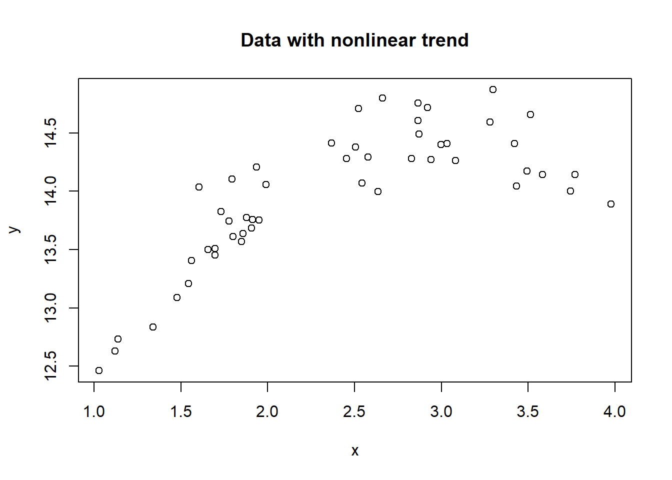
The first few rows of data looks like this
##          y        x
## 1 12.83440 1.341110
## 2 14.60609 2.866898
## 3 14.28045 2.827824
## 4 14.48854 2.870138
## 5 14.14301 3.582746
## 6 14.71733 2.920932
Obviously, fitting a straight line (a linear model in \(x\)) does not make sense. From the scatterplot, we might consider a second order polynomial to be realistic, so we look to estimate based on the model
\[ y = \beta_0 + \beta_1 x + \beta_2 x^2 + \mathcal{E}\;. \]
According to the method outlined above, we can do this by simply adding a column x_sq containing the values of \(x^2\) to the dataframe, and then run a regression of y on x and x_sq. $r_sq
Here is the R code for this.
##          y        x      x_sq
## 1 12.83440 1.341110  1.798577
## 2 14.60609 2.866898  8.219105
## 3 14.28045 2.827824  7.996590
## 4 14.48854 2.870138  8.237694
## 5 14.14301 3.582746 12.836070
## 6 14.71733 2.920932  8.531843
Now run the regression:
## (Intercept)           x        x_sq
##   9.6155026   3.2886803  -0.5555102
So the estimated model is \[ y = 9.62 + 3.289 x - 0.556 x^2\;. \] Note that the coefficients are close - but not equal - to the values used in simulation. The differences are caused by our adding random error in the simulation. Now, let us plot the data, with the fitted 2nd order curve, as well as the (bad) linear model trend.
badreg <- lm(y ~ x, data = DF)
with(DF, plot(x, y, main = "Data with fitted linear and nonlinear trend."))
abline(badreg, col = "black")
curve(9.62 + 3.298*x - 0.556*x^2,
      add = TRUE,
      col = "blue",
      lwd = 2)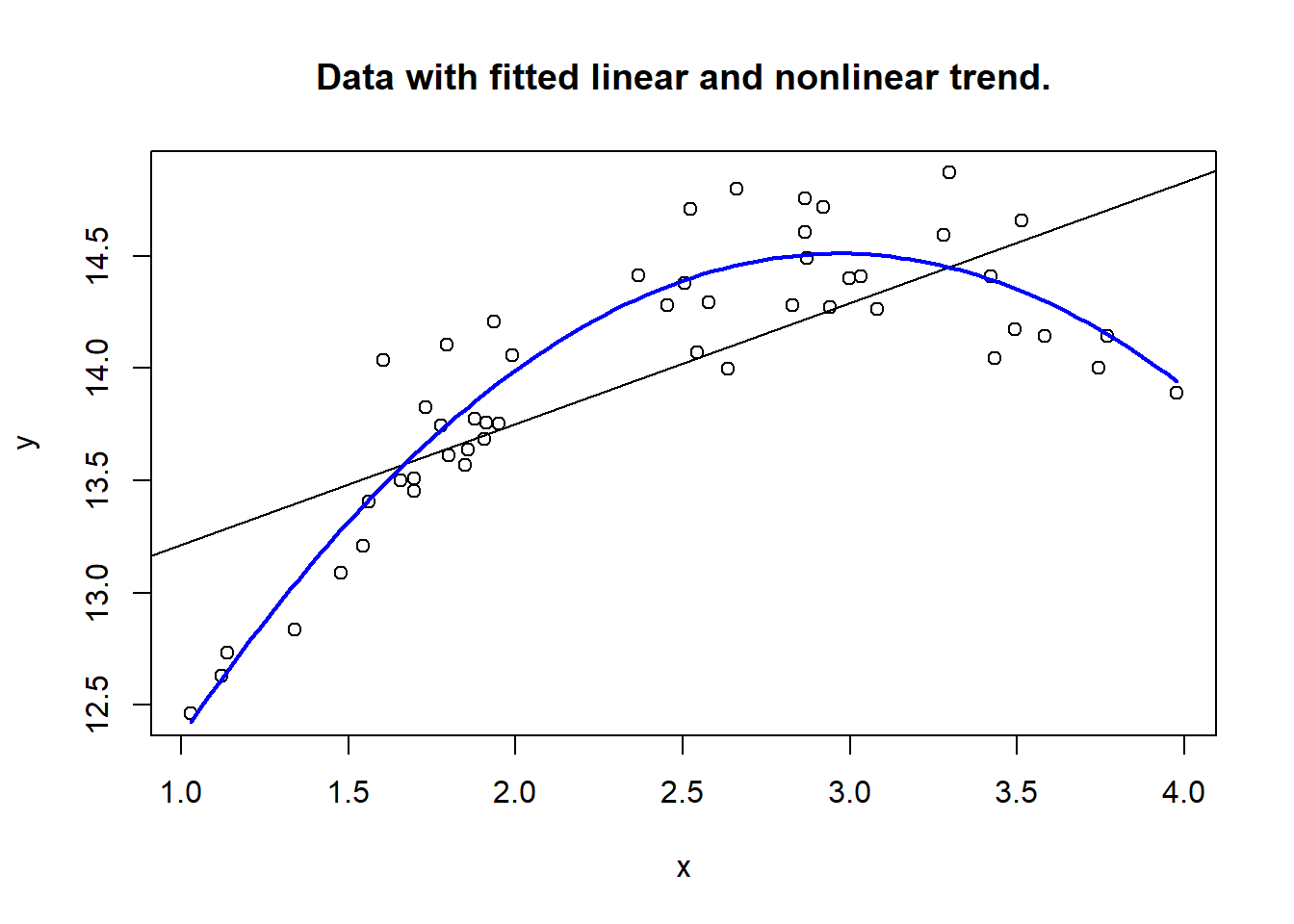
:::
7.2.1 An alternative approach with R.
We have chosen to outline the method above in general, since this is the way one can handle such non-linearities in most statistical software. R does however provide a more direct way to estimate such type of models, and this involves a trick with the regression formula in the lm function. Just following the simulation example above, we could actually work on the original dataframe with \(x\) and \(y\) and force R to estimate the 2nd order term as follows
##          y        x
## 1 12.83440 1.341110
## 2 14.60609 2.866898
## 3 14.28045 2.827824
## 4 14.48854 2.870138
## 5 14.14301 3.582746
## 6 14.71733 2.920932
Now, estimate with the following code
## (Intercept)           x      I(x^2)
##   9.6155026   3.2886803  -0.5555102
The term I(x^2) tells R to include \(x^2\) as a new variable, but it will not be actually stored in any dataframe with this method.
In fact, for anyone who works regularly with R, this is the preferred way of doing such models.
Note that the I(...) is neccessary here, it will not work to use something like
##
## Call:
## lm(formula = y ~ x + x^2, data = DF)
##
## Coefficients:
## (Intercept)            x
##     12.6759       0.5384
7.3 Categorical variables in regression - Dummy variables
Perhaps the most common non-linear effect in regression models comes when we want to
include categorical variables. This is something we commonly want to do, whenever a
categorical factor is suspected to affect our dependent variable. To illustrate the method
for handling such factors, let us consider models for flat prices in Molde, Ålesund and Kristiansund.
For simplicity, let \(X_1\) denote the floorspace area of sold flats, and let \(X_2\) be the variable
encoding town location. In the data set flat_prices.csv, the encoding is
\[ X_2 =
\left\{
\begin{array}{ll}
1, & \hbox{for Molde;} \\
2, & \hbox{for Kristiansund;} \\
3, & \hbox{for Ålesund.}
\end{array}
\right.
\]
Let us load the data, and have a look at what we try to accomplish in this section. To easily visualize what we are looking to model, we now use the ggplot2 package here.
library(ggplot2)
#load data
flatprices <- read.csv("Data/flat_prices.csv")
#plot price vs area relation for each town, with separate regression lines.

ggplot(flatprices, aes(x = area, y = price, color = factor(town))) +
        geom_point(size=2) +
        geom_smooth(method = lm, se = FALSE) +
        labs(title = "Price vs area in three towns")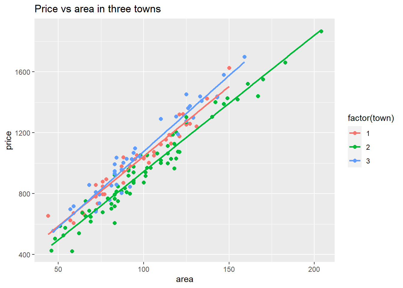
Figure 7.1: Visualizing differences between towns
What we see here is that the prices increase with area in almost the same way in the three towns, but there appears to be some difference in the general level, in particular town = 2 (Kristiansund) shows generally lower prices. How can we model this and estimate the observed differences?
Obviously, the encoding by \(X_2\) as 1, 2, 3 is completely arbitrary, and even redundant. Taking \(X_2\) directly into a regression model as a linear term is just leading to a “crazy” model as we will see: If we define our model as \[\begin{equation} Y = \beta_0 + \beta_1 X_1 + \beta_2 X_2 + \mathcal{E}\;, \tag{7.3} \end{equation}\] we are implicitly assuming the following about the average prices \(Y_{mean}\) given area \(X_1\):So, this (crazy) model supposes some parameter \(\beta_2\) which is the difference in general price level between Kristiansund and Molde. At the same time \(\beta_2\) is also the difference between levels in Ålesund and Kristiansund. It makes sense to suspect differences in average price levels between towns, but there is absolutely no reason to assume that the differences are the same, as the above model implies. In addition, we realize that the numerical encoding could simply be absent in the data so that only town names would appear. Then the idea that we can just assign some encoding 1, 2, 3 - and then expect prices to depend linearly on this - is far from realistic! We will need to do it differently. We will use “dummy variables”.
7.3.1 Dummy variables
A dummy variable is a variable that only takes the values 0 or 1. We use such variables to indicate whether a condition is true or false for an object. The value 1 indicates true. In the flat price example we could define three dummy variables \(D_1, D_2, D_3\) as follows.
- \(D_1 = 1\) if the flat is in Molde, otherwise, \(D_1 = 0\).
- \(D_2 = 1\) if the flat is in Kristiansund, otherwise, \(D_2 = 0\).
- \(D_3 = 1\) if the flat is in Ålesund, otherwise, \(D_3 = 0\).
So, each of the dummy variables indicates whether a flat belongs to the particular town with which it is associated. Now, it turns out to work well if we include these variables into the regression model. However, we shall only include two of them. In fact, you realize that there is complete linear dependence among the three variables, so we may write \[ D_3 = 1 - D_2 - D_1\;. \] Including all three would simply violate the fundamental assumption (E) about linear dependence among independent variables. So, for a categorical variable with three groups as in this example, we will use two dummy variables to encode the information. The choice of which dummy variable to leave out is usually not important. We will see that the “left out group” serves as a reference group, and we may estimate correction coefficients for the other groups. So suppose we want to use Molde as our reference group. Then we define the model as \[\begin{equation} Y = \beta_0 + \beta_1 X_1 + c_2 D_2 + c_3 D_3 +\mathcal{E}\;, \tag{7.4} \end{equation}\] where \(c_2, c_3\) are two new coefficients. Since we assume the error term has mean 0, this model assumes the mean price given the involved variables is \[ Y_{mean} = \beta_0 + \beta_1 X_1 + c_2 D_2 + c_3 D_3\;.\] So, let’s see what this means for the three towns.
- For a flat in Molde, \(D_2 = D_3 = 0\), so \[ Y_{mean} = \beta_0 + \beta_1 X_1 \;, \]
- For a flat in Kristiansund, \(D_2 = 1, D_3 = 0\), so \[ Y_{mean} = \beta_0 + \beta_1 X_1 + c_2 = (\beta_0 + c_2) + \beta_1 X_1\;, \]
- For a flat in Ålesund, \(D_2 = 0, D_3 = 1\), so \[ Y_{mean} = \beta_0 + \beta_1 X_1 + c_3 = (\beta_0 + c_3) + \beta_1 X_1\;. \]
All of this means that there is a basic linear relation between area and prices expressed by a common (marginal) square meter price \(\beta_1\). What is different in the three towns is the constant term. As we see, the coefficients \(c_2, c_3\) has the effect of adjusting the basic price level from Molde to the two other towns. This allows us to operate with two completely independent corrections to the price level in Molde. This was not the case with the original model (7.3).
We end this section with the general remark that we will need \(k-1\) dummy variables in order to represent a categorical variable with \(k\) different values in a regression model. The omitted value serves as a reference group. For all other groups, an adjusting coefficient represents the difference relative to the reference group.
7.3.2 Computing dummy variables in R
Usually, our data material will include categorical variables in their
original form, i.e. a single variable with for example three distinct
values. The values can be numerical like 1, 2, 3. For nominal variables the values can be just
names of categories. For the flat price example, there is a numerical
encoding of the town variable, but this encoding has little purpose apart from being
faster to type initially. For use in regression models, we need to create dummy variables
for all but one value of a categorical variable. In R we can simply use logical expressions to compute
dummy variables. So let us consider the flat prices data, and create dummy variables DKSU and DASU indicating
with value 1 that a flat is in Kristiansund or Ålesund. In doing so, we use the common practice in programming languages
that a logical value TRUE/FALSE naturally corresponds to integer values 1/0. So we can do the following with our
flatprices dataframe:
#encode DKSU = 1 for Kristiansund
flatprices$DKSU = as.integer(flatprices$town == 2)
#encode DASU = 1 for Ålesund
flatprices$DASU = as.integer(flatprices$town == 3)
#show first/last 4 rows:
rbind(head(flatprices, 4),  tail(flatprices, 4))
## price area rooms standard situated town distcen age rent DKSU DASU
## 1 1031 100 3 2 6 1 5 15 2051 0 0
## 2 1129 116 3 1 5 1 4 42 2834 0 0
## 3 1123 110 3 2 5 1 3 25 2468 0 0
## 4 607 59 2 3 5 1 6 25 1940 0 0
## 147 810 72 2 1 2 3 1 15 1785 0 1
## 148 1069 94 3 2 6 3 1 47 2043 0 1
## 149 1028 90 2 3 6 3 4 30 1455 0 1
## 150 1003 88 3 3 8 3 4 25 1919 0 1Here we see the idea, for flats in Molde, both dummy variables are 0, for flats in Ålesund we see DKSU = 0, DASU = 1.
7.3.3 Continuing the flat prices example in R.
In chapter 6 we had a first look at some multiple regression models for how flat prices \(Y\) depends on various attributes of the flats. If we extend our experiment with a straight linear model, we could try predictor variables among the following
- Area
- Flat location (rated 0-10) (the variable is called
situated) - Distance to town center in Km
- Age of flat
- Number of rooms
- monthly fixed cost. (the variable is called
rent).
From a modeling perspective, one could argue that even some of these variables should be recoded into
dummy variables. However, these variables are at least ordinal, and assuming
a near linear dependency is not unreasonable. With the aim of keeping simplicity we keep these variables in original form.
Let’s compare three models here: A using only area, B using all the variables, C using all variables from B that was significant.
We will look at these, particularly with a focus on the \(R^2\) and the \(S_e\) results, which tells something about the predictive power of the models. We use the update function described in section 6.3.1, to effectively adjust the models we work on:
library(stargazer)
#run regressions: start with basic model A, then update in two steps.
flatregA <- lm(price ~ area, data = flatprices)
flatregB <- update(flatregA, . ~ . + situated + distcen + age + rooms + rent) #add variables
flatregC <- update(flatregB, . ~ . - age - rooms) #remove two.
#show results
stargazer(flatregA, flatregB, flatregC,
          type = "text",
          keep.stat = c("rsq", "ser" ),
          column.labels = c("A", "B", "C"),
          model.numbers = FALSE)
##
## =========================================================================
## Dependent variable:
## -----------------------------------------------------
## price
## A B C
## -------------------------------------------------------------------------
## area 9.130*** 10.407*** 9.860***
## (0.246) (0.417) (0.171)
##
## situated 18.082*** 17.873***
## (2.763) (2.766)
##
## distcen -24.060*** -23.931***
## (2.521) (2.525)
##
## age -0.421
## (0.611)
##
## rooms -14.449
## (10.023)
##
## rent -0.096*** -0.097***
## (0.009) (0.009)
##
## Constant 93.697*** 210.911*** 213.640***
## (25.332) (31.425) (24.990)
##
## -------------------------------------------------------------------------
## R2 0.903 0.964 0.963
## Residual Std. Error 88.519 (df = 148) 54.906 (df = 143) 55.033 (df = 145)
## =========================================================================
## Note: *p<0.1; **p<0.05; ***p<0.01So, what we see here is that in model A, we get \(S_e = 88.5\), while in model B, C (with more predictor variables) we improve to \(S_e\) close to 55. From section 6.5 we recall the approximate 95% error margin for predictions is \(2S_e\), so moving from model A to C, we improve prediction errors from about 177 to 110.
Next, now we want to include the categorical variable town in the form of the two dummy variables DKSU, DASU, and see if we can further improve the prediction power. We will now look at two additional models, and try to understand the role of the dummy variables here:
- model D: extend model A above withthe two dummy variables
- model E: extend model C above with the two dummy variables.
#update model A
flatregD <- update(flatregA, . ~ . + DKSU + DASU)
#update model C
flatregE <- update(flatregC, . ~ . + DKSU + DASU)

#look at new results:
stargazer(flatregA, flatregD, flatregC, flatregE,
          type = "text",
          keep.stat = c("rsq", "ser" ),
          column.labels = c("A", "D", "C", "E"),
          model.numbers = FALSE)
##
## ===========================================================================================
## Dependent variable:
## -----------------------------------------------------------------------
## price
## A D C E
## -------------------------------------------------------------------------------------------
## area 9.130*** 9.223*** 9.860*** 9.978***
## (0.246) (0.185) (0.171) (0.033)
##
## DKSU -100.538*** -106.013***
## (13.075) (2.095)
##
## DASU 30.910** 2.665
## (14.850) (2.419)
##
## situated 17.873*** 15.779***
## (2.766) (0.536)
##
## distcen -23.931*** -21.160***
## (2.525) (0.496)
##
## rent -0.097*** -0.098***
## (0.009) (0.002)
##
## Constant 93.697*** 123.371*** 213.640*** 254.281***
## (25.332) (20.520) (24.990) (5.056)
##
## -------------------------------------------------------------------------------------------
## R2 0.903 0.946 0.963 0.999
## Residual Std. Error 88.519 (df = 148) 66.350 (df = 146) 55.033 (df = 145) 10.617 (df = 143)
## ===========================================================================================
## Note: *p<0.1; **p<0.05; ***p<0.01Firstly, we can compare model A to model D. What model D does is to allow for price corrections between the towns. From the regression we see that those effects are highly significant, with Kristiansund being about 100 000 lower, Ålesund about 30 000 higher than Molde, when we do not control for other factors. Those numbers correspond closely to the vertical difference between the lines in figure 7.1. (e.g. the green line is about 100 units below the orange one.) We can see that inclusion of the dummy variables substantially improves the prediction precision (as measured by \(S_e\) = Residual Std. Error).
Now looking at the more refined models to the right, we see that with the inclusion of other variables, DASU is not really significant, while DKSU remains a highly significant variable. Alltogether in model E we achieve a major improvement of predictive precision, as we see comparing to model C here. The 95% margin of error for predictions is down to about 20 000 with this model. So the bottom line is that including categorical variables in regression can be of great importance for the quality of the model.
Thus we have seen one way of including categorical information into regression analyses. This method is general enough to be used also if you should prefer other statistical tools than R.
7.4 Interaction effects
Non-linear effects in regression can often be modeled using products of variables. As an example, consider modeling intra-city route duration \(Y\) for parcel delivery & pick-up routes. A vehicle has a route with a certain number of stops for delivery and/or pick-up. The route has a certain total distance. In addition the model should take into account two different levels of traffic: “rush-hour” and “normal”. Clearly, the route duration \(Y\) depends on all of these factors:
- Number of stops, which we call \(X_1\),
- Total distance (km) which we call \(X_2\),
- Traffic level.
Ignoring the traffic level, we could reasonably model the \(Y\) dependency on \(X_1, X_2\) as a linear model, \[\begin{equation} Y = \beta_0 + \beta_1 X_1 + \beta_2 X_2 + \mathcal{E}\;. \tag{7.5} \end{equation}\] In this model, the interpretation of parameters is straightforward. The \(\beta_1\) represents the average duration of a pick-up/delivery stop, while \(\beta_2\) describes the average driving time pr. km. However, some important information is not utilized in the (7.5) model. Since we are operating with two different traffic situations, we would expect durations of equal-length routes to be higher in rush-hour conditions than in normal traffic. How could we reasonably model this? Since we now know about dummy variables, and the traffic level is a categorical variable with only two values, we should encode this as a dummy variable, with for example the normal level as reference level, i.e. define a variable \(H\) (for High traffic) by \[ H = \left\{ \begin{array}{ll} 0, & \hbox{if normal traffic;} \\ 1, & \hbox{if rush-hour traffic.} \end{array} \right. \] How would this variable affect route duration? Suppose we include \(H\) with a coefficient \(\beta_H\) directly into the model, as a separate term: \[\begin{equation} Y = \beta_0 + \beta_1 X_1 + \beta_2 X_2 + \beta_H H + \mathcal{E}\;. \tag{7.6} \end{equation}\] Can you see what \(\beta_H\) represent in this model, and maybe why this is not a realistic description of the situation?
A more realistic approach, is to assume that the actual average driving time pr. km. changes when we switch from normal to rush-hour traffic conditions. In terms of model (7.5) this would mean that we should allow the \(\beta_2\) coefficient to be adjusted depending on traffic level. So, we include the dummy variable \(H\) in the following way: \[\begin{equation} Y = \beta_0 + \beta_1 X_1 + (\beta_2 + \beta_H H) X_2 + \mathcal{E}\;. \tag{7.7} \end{equation}\] Since \(H\) can only be 0 or 1, we can write out exactly what the model states in each case.
- If normal traffic, \(Y = \beta_0 + \beta_1 X_1 + \beta_2 X_2 + \mathcal{E}\;.\)
- If rush hour traffic \(Y = \beta_0 + \beta_1 X_1 + (\beta_2 + \beta_H) X_2 + \mathcal{E}\;.\)
The \(\beta_H\) variable simply corrects the way \(X_2\) affects \(Y\), depending on traffic level. This is often called an interaction effect. The variables \(X_2\) and \(H\) interacts in the way they impact on route duration \(Y\). The effect of the \(H\) variable is easiest to see in the direct form (7.7) of the model. For practical (estimation) purposes, however, we may need to rewrite the model slightly: \[\begin{equation} Y = \beta_0 + \beta_1 X_1 + \beta_2 X_2 + \beta_H (H \cdot X_2) + \mathcal{E}\;. \tag{7.8} \end{equation}\] This model uses three variables, \(X_1, X_2\) and the new variable \(H \cdot X_2\) which is simply the product of \(H\) and \(X_2\). To make it explicit, we define a new variable \(X_H\) by \[ X_H = H \cdot X_2\;.\] Then the model reads \[\begin{equation} Y = \beta_0 + \beta_1 X_1 + \beta_2 X_2 + \beta_H X_H + \mathcal{E}\;. \tag{7.9} \end{equation}\] In this, note again that (7.9) is a linear model in the three variables \(X_1, X_2, X_H\), while the formulation in (7.7) is a nonlinear model in the three variables \(X_1, X_2, H\).
For practical purposes, in R (or other software), we would compute values for the new variable \(X_H\) and run a linear regression on model (7.9) to obtain parameter estimates for \(\beta_0, \beta_1, \beta_2, \beta_H\). In fact the practical handling of the interaction effect is the same as we described in section 7.2, since it ultimately results in a model involving a product of variables.
7.5 An alternative with R - using factor representation.
As mentioned above, we chose to use the general method with dummy variables to incorporate categorical variables in regression. However, R offers a nice alternative which is the “standard” method in R and other advanced statistical languages. This is done by allowing a categorical variable to be defined as a factor. We touched upon the concept of a factor in section 3.6.8. Essentially, a factor is a character vector with an additional set of levels which are all possible values the vector can have.
We will continue with the flatprices dataframe as an example of this method. We will be using the recode function from the package dplyr briefly here to recode a little bit.
library(dplyr)
#redefine town as character:
flatprices$town <- as.character(flatprices$town)
#recode to names "Molde", "Krsund", "Alesund":
flatprices$town <- recode(flatprices$town, "1" = "Molde", "2" = "Krsund", "3" = "Alesund")
#define town as "factor".
flatprices$town <- factor(flatprices$town, levels = c("Molde", "Krsund", "Alesund"))
#check the structure
str(flatprices)
## 'data.frame': 150 obs. of 11 variables:
## $ price : int 1031 1129 1123 607 858 679 1300 1004 673 1187 ...
## $ area : int 100 116 110 59 72 64 129 103 59 115 ...
## $ rooms : int 3 3 3 2 2 2 4 3 2 3 ...
## $ standard: int 2 1 2 3 3 2 1 2 2 1 ...
## $ situated: int 6 5 5 5 4 3 5 5 5 6 ...
## $ town : Factor w/ 3 levels "Molde","Krsund",..: 1 1 1 1 1 1 1 1 1 1 ...
## $ distcen : int 5 4 3 6 1 3 3 3 1 5 ...
## $ age : int 15 42 25 25 17 17 32 17 27 15 ...
## $ rent : int 2051 2834 2468 1940 1611 2039 2708 2981 2372 2126 ...
## $ DKSU : int 0 0 0 0 0 0 0 0 0 0 ...
## $ DASU : int 0 0 0 0 0 0 0 0 0 0 ...We see that town is now a factor. The effect of this is that we can simply include the variable into a regression formula, and R will automatically do all the “dummy variable stuff” behind the scenes. Here is how we would estimated model D from above with this method.
#replicate model D: (save as F)
flatregF <- lm(price ~ area + town, data = flatprices)
#check the results:
summary(flatregF)
##
## Call:
## lm(formula = price ~ area + town, data = flatprices)
##
## Residuals:
## Min 1Q Median 3Q Max
## -181.358 -41.656 -8.524 47.070 145.821
##
## Coefficients:
## Estimate Std. Error t value Pr(>|t|)
## (Intercept) 123.3706 20.5204 6.012 1.40e-08 ***
## area 9.2232 0.1846 49.952 < 2e-16 ***
## townKrsund -100.5377 13.0755 -7.689 2.01e-12 ***
## townAlesund 30.9100 14.8497 2.082 0.0391 *
## ---
## Signif. codes: 0 '***' 0.001 '**' 0.01 '*' 0.05 '.' 0.1 ' ' 1
##
## Residual standard error: 66.35 on 146 degrees of freedom
## Multiple R-squared: 0.9463, Adjusted R-squared: 0.9452
## F-statistic: 857.5 on 3 and 146 DF, p-value: < 2.2e-16We see that this is identically the same model. The way we defined levels for our factor made “Molde” into the reference category, as we did with the dummy variables. Using factors in this way is certainly the recommended method if one is to work further with regression models in R.