Chapter 4 Hypothesis testing
In this chapter we take on the basics of hypothesis testing, which is the core activity in inferential statistics. We will establish the general terminology and the basic principles. We will then discuss some specific tests, and show how to work those out with R.
4.1 Testing statistical hypotheses
In general, a statistical hypothesis is a statement about some “populations”, “system” or “reality”.
Such hypotheses can often be formulated in terms of some parameters of a population (or of a system). The theory of hypothesis testing uses statistical methods to asses the validity (truth) of such hypotheses. We need statistical methods in cases where the populations or system is too large or complex for a complete examination, i.e. we have only a sample of information to base our assessment on.
Although hypotheses comes in a variety of forms and settings, there is a general way of performing tests of the validity. This chapter will focus on this general idea, with a few basic examples of application. Every other hypothesis test you see in this text, will be using the same principles.
Let us see a few informal examples of hypotheses as statements, and their parametric form.
We consider the following example.
Example 4.1 (Hypothesis examples.)
- Hypothesis: “The selling prices of houses in Norway increased from April to May 2013.” If \(\mu_x\) and \(\mu_y\) are the mean square meter prices for sold houses, in April and May respectively, we would get the parametric form \[ \mu _y > \mu_x \] of the hypothesis. Here the “system” is the Norwegian housing market, and populations are all sold houses in April and May respectively. The hypothesis is clearly a statement about that system (and those populations).
- Hypothesis: “The minced meat from the producer ACNE FOOD exceeds the legal maximum fat content of 10%.” If \(\mu\) is the mean fat content in packets from ACNE, we would get the parametric form \[ \mu > 10 \] for this hypothesis. We consider the population in this case as all packets coming from ACNE within the current production period.
- Hypothesis: “The proportion of buying customers among visitors to a web-shop has increased with a new web solution for the shop.” Assuming the proportion used to be \(p_0 = 0.13\) and is now an unknown parameter \(p\), we get the parametric form \[ p > 0.13 \] A verification of the hypothesis would indicate that the redesign of the web site was successful. (In real life, we would ask for a little more than just to increase the proportion from 0.13. What would really matter is whether income increase will cover the investment cost of the redesign.)
Regarding the example, if we were to assess validity of those hypotheses with sample information, our data would likely be
- Samples of square meter prices of sold houses for the two months.
- A sample of fat contents for a number of packets of meat.
- Sample of visiting customers, along with information of whether they bought or not.
We would have to use the relevant parameter estimates in each case, to seek possible support for the hypothesis. In each of the cases, that would be
- The (sample) mean prices from each month \(\bar{x}, \bar{y}\) and the (sample) standard deviations of the prices (\(S_x, S_y\)).
- The mean and standard deviation (\(\bar{x}, S_x\)) of the sampled fat contents.
- The sample proportion \(\hat{p}\) of buyers.
In addition to the values of parameter estimates, also the sample sizes will be important when we seek evidence for a hypothesis. Still with reference to the examples 1 - 3 above, we will learn how to answer questions like the following.
- Suppose the sample mean square meter prices were \(\bar{x} = 19800\) in April, and \(\bar{y} = 20100\) in May, with sample sizes 300 and 200 respectively. Suppose the standard deviations of prices were \(S_x = 350\) and \(S_y = 410\). Clearly, the mean price in the samples was higher in May. Could that be just coincidental, or do we have real evidence of a true change in price level?
- Suppose we sample \(n=50\) packets of the ACNE meat, and find a mean fat content of \(\bar{x} = 11\%\), with standard deviation \(S_x = 0.9\%\). Clearly, the sample mean is somewhat above the legal limit at 10%. Is this a strong evidence for the hypothesis \(\mu > 10\)?
- Suppose we find sample proportion of buyers \(\hat{p} = 0.16\) from a sample of \(n = 400\) customers. Clearly, this points in the direction of the hypothesis, but is it hard evidence that the real proportion \(p\) is above 0.13?
The answers are 1) yes, 2) yes and 3) no. We will come back to each of these examples later.
In each case, the randomness of the sampling process makes it possible that the hypothesis is actually false, and that the results we see are just coincidentally supporting the hypotheses. However, as we will see, in case a) and b) it is extremely unlikely that the sample results are caused by mere coincidence. In case c) on the other hand, the sample result may well be seen in a situation where \(p=0.13\), i.e. where the claimed hypothesis is false.
4.2 A motivating example
Let us focus on the example 2) above. We will try to pin down the fundamental ideas for a hypothesis test in this setting, with a minimum of technical detail. Following the conventions of testing, the test in this example would be written as follows. \[\begin{equation} H_0: \mu \leq 10 \ \mbox{vs.} \ H_1: \mu > 10. \tag{4.1} \end{equation}\]
In this setting, \(H_0\) is called the null hypothesis, and \(H_1\) is called the alternative hypothesis. We are interested in whether sample information \[ n, \quad \bar{x},\quad S_x \] gives strong reason to believe that \(H_1\) is true. Note that evidence for \(H_1\) is the same as evidence against \(H_0\) in this case.
Assume for now that \(n = 50\) and \(S_x = 0.9\) as in the example. Let us consider some possible values for the sample mean. Clearly, if \[ \bar{x} \leq 10, \] we have absolutely no reason to believe that \(H_1\) is true. If \(\bar{x} = 10.01\) we would say that we have a very weak indication of \(H_1\), because in this case it is quite likely that \(H_0\) is true and that randomness in the sampling causes \(\bar{x}\) to exceed the value 10. But what if \(\bar{x} = 10.1\)? or \(10.5\)? Or \(11\)? It is difficult to judge these cases intuitively. We need some theory.
Thinking of this example, we naturally look at the difference \[ \bar{x} - 10. \] If this is positive, we agree that the sample information points towards \(H_1\). If the value is “small”, we would suspect that the sample result could be coincidental. If the value is “large”, we would suspect that this can only be because \(H_1\) is true. Still, at this point, we do not exactly know what will be a “small” and a “large” value. The key concept to get to the next level here, is that of a test statistic. For this particular example, we should use the following expression \[\begin{equation} T = \frac{\bar{x} - 10}{S_x/\sqrt{n}} = \frac{\bar{x} - 10}{0.9/\sqrt{50} } \;, \tag{4.2} \end{equation}\] as our test statistic.
If you now recall our brief discussion of sampling distributions in section 2.8
you will remember that we can consider \(\bar{x}\) as a random variable. Then \(T\) is also a random variable. Now, the whole key to answer our questions lies in the fact that we may know the probability distribution of \(T\) - given that \(H_0\) is true. In this example, we will find that \(T\) is very near standard normal distributed (if \(H_0\) is true). This has some interesting consequences. Given the specific values for \(\bar{x}, S_x\) and \(n\) we call the resulting value on \(T\) the observed T value.
We write \(T_{_{OBS}}\) for this value. The table below summarizes our example values for \(\bar{x}\) and \(T_{_{OBS}}\).
| \(\bar{x}\) | 10.01 | 10.10 | 10.50 | 11.00 |
| \(T_{_{OBS}}\) | 0.079 | 0.786 | 3.928 | 7.857 |
Let’s agree that the value of \(T_{_{OBS}}\) is more in favor of \(H_1\) the larger it is. (Because larger \(T_{_{OBS}}\) comes along with larger \(\bar{x}\)). So the values in the table gives increasingly strong evidence of \(H_1\) as we move right.How strong the evidence is can be measured by recalling that \(T\) is standard normal if \(H_0\) is true (and thus \(H_1\) false). Now, if \(T\) is standard normal, is the observation \[ T_{_{OBS}}= 0.079 \] remarkable? Clearly not, since this observation is almost at 0, the expected value for \(T\). It means the observation gives no reason to doubt \(H_0\). What about \[T_{_{OBS}}= 0.786\;? \] Well, if \(T\) is standard normal we know that typical values are between \(\pm 2\) with more probability centered close to 0. The value 0.786 is completely in line with the assumption that \(T\) is standard normal, i.e. that \(H_0\) is true.
(Look to figure 4.1 to see how the value fits with the distribution).
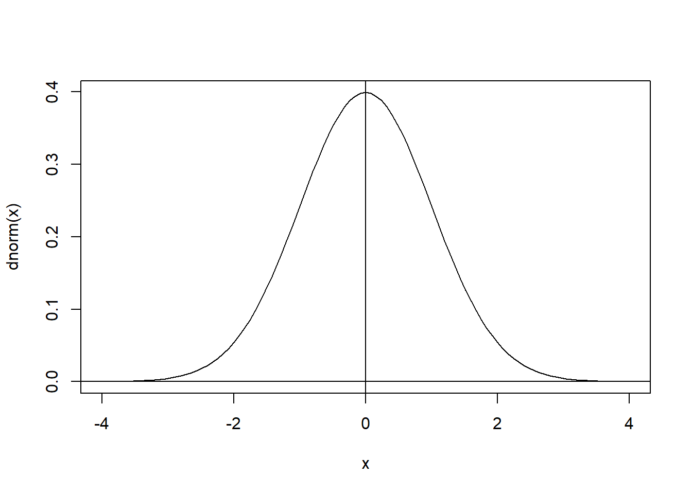
Figure 4.1: The standard normal distribution
We would not say that \(T_{_{OBS}}= 0.786\)
gives strong evidence against \(H_0\) - and thus no strong evidence for \(H_1\). Now, consider the value
\[ T_{_{OBS}}= 3.928\; . \]
This is a different situation. Our work on the standard normal distribution taught us that it becomes increasingly improbable to see values beyond 2
for this distribution, and our value here is close to 4. The probability of seeing \(T\) at this value - or higher - is
practically speaking zero. (It is about 0.000032, try with R: 1 - pnorm(4))
Ok, so if you tell me that the variable \(T\) came out with the value 3.928, I refuse to believe that \(T\) is a standard normal variable. But if \(H_0\) is true, it should be! - OK, so I refuse to believe in \(H_0\). I claim to have strong evidence against \(H_0\). I have seen something that would be almost impossible if \(H_0\) was true, so I refuse to believe in it. We will measure the strength of this evidence for \(H_1\) exactly by the probability \[ P[ T \geq T_{_{OBS}}] \ \ \mbox{given that $H_0$ is true.} \] This probability is called the \(P\)-value of the observation \(T_{_{OBS}}\) for this test. Here the \(P\)-value is 0.000032. The lower the \(P\)-value, the stronger we consider the evidence.
Continuing, we realize that the observation of \(T_{_{OBS}}\) at 7.857 is even more extremely contradicting the null hypothesis, since such a value will practically never appear for a standard normal variable.
To summarize, we arrive at the conclusion that none of the \(\bar{x}\) values at 10.01 or 10.1 gives real evidence for \(\mu > 10\), while both of the values 10.5 and 11.0 gives very solid evidence. Note carefully how the observed value of \(T\) is used when we try to “contradict” \(H_0\). If the observed value is very improbable for the distribution given true \(H_0\), we must conclude that \(H_0\) is probably not true.
4.3 The testing framework
We now move on to a more formal outline of the hypothesis testing framework. The concepts that we will review, are the following.
- Null hypothesis \(H_0\) and alternative hypothesis \(H_1\).
- Test statistic and its distribution given \(H_0\).
- Critical direction and \(P\)-value.
- Significance level and rejection of null hypothesis.
- The difference between \(H_0\) and \(H_1\)
- Type I and Type II error
The first three concepts should be easily recognizable from the previous example.
4.3.1 Null hypothesis and alternative hypothesis
The alternative hypothesis \(H_1\) is a claim about populations, systems or reality as described above. In statistics we deal with the parametric form of the hypotheses. We focus here on the case where we have only one parameter. All examples shown here are of this type. Let us be general, and call the parameter \(\beta\). So, \(\beta\) is a number describing some property of, say, a population. (It could be a mean, a proportion, a standard deviation and so on.) In interesting cases, \(\beta\) will be unknown. Otherwise we would not need statistics. In almost all cases, the \(H_1\) hypothesis will have one of the following forms, where \(b\) is a particular fixed number. \[ \beta > b, \quad \beta < b, \quad \ \mbox{or} \ \beta \ne b \;. \] Opposing \(H_1\) is the null hypothesis, \(H_0\). This represents something contrary to \(H_1\), so if \(H_1\) states \[ \beta > b \] then \(H_0\) will be one of the following: \[ \beta = b \ \mbox{or} \ \beta \leq b \;.\] Statistically, these two forms are treated in identical manner. It is technically easier to work with the form \(\beta = b\), so we start there. When the alternative and null hypotheses are clear, we usually write them together as for instance \[ H_0: \beta = b \ \mbox{vs.} \ H_1: \beta > b\;. \] Now, the idea is that we will try to “prove” the truth of \(H_1\). To do that, we need to observe a sample from the population in question. Since \(\beta\) is a parameter of the population, the sample will provide an estimate for \(\beta\) and (directly or indirectly), this estimate can be used to judge whether we believe \(H_1\) is true (and \(H_0\) false). The estimate of \(\beta\) is usually part of an expression we call the test statistic. To give a concrete example, recall the hypotheses in equation (4.1). Here the parameter \(\beta\) is the mean \(\mu\), the fixed number \(b\) is 10, the estimate for the parameter is \(\bar{x}\) and this is indirectly used in the expression of the test statistic in equation (4.2).
4.3.2 The test statistic, critical direction and \(P\)-value
We consider a test where the null hypothesis is on the form \[ \beta = b \] and the alternative is one of the three possibilities mentioned above. We suppose we have a sample from the population. The test statistic is a quantity \(T\) that has the following properties.
- \(T\) has a known probability distribution given that \(H_0\) is true.
- \(T\) is computable from the sample.
Looking back at the example in section 4.2, the test statistic is called \(T\), it has a standard normal distribution when \(H_0\) is true, and it is clearly computable from the sample. As we see in that example, it is the observed value of \(T\) that ultimately decides the test.
The whole idea of how we use a test statistic \(T\) is as follows. First, let us say that of two possible observed values \(a, b\) for \(T\), \(a\) is more critical than \(b\) if observing \(T_{_{OBS}}= a\) gives stronger evidence for \(H_1\) than observing \(T_{_{OBS}}= b\). Although somewhat abstract at this point, it is usually easy to say what is more critical in a specific given test. In the example in section 4.2, a larger value for \(T_{_{OBS}}\) is more critical.
The conclusion of the test follows the steps below.
- Step 1: Compute the observed value \(T_{_{OBS}}\).
- Step 2: Using the probability distribution for \(T\), find the \(P\)-value, i.e. the probability that \(T\) would have a more critical value than \(T_{_{OBS}}\), given that \(H_0\) is true.
- Step 3: If the \(P\)-value is sufficiently low, we conclude that it is unlikely that \(H_0\) is true, so we reject \(H_0\) in favor of \(H_1\).
In practical statistics, we routinely use software to perform steps 1 and 2, so as to get a \(P\)-value. Then the \(P\)-value is used to make the judgement in step 3. We will return shortly to what we mean by “sufficiently low”.
4.3.3 Significance level
The statement in step 3 above needs some more precision. In testing statistical hypotheses, it is common to employ a significance level. This is a pre-specified probability often called \(\alpha\). Typical values are 0.05 or 0.01. If the significance level is set, say at \(\alpha = 0.05\), we perform step 3 as follows. If the \(P\)-value is less than \(\alpha\) we reject \(H_0\) in favor of \(H_1\). We then say that we have significant evidence for the alternative hypothesis, or that the conclusion that “\(H_1\) is true” is significant at level 0.05. Clearly, the lower the \(P\)-value, the stronger is the evidence for \(H_1\). Recall the very small values in the previous motivating example.
If you find this outline hard to comprehend, you will find that it is still possible to use R in a relatively “automatic” way for testing. Essentially, you need to select the right kind of test, run with R, and check the \(P\)-value.
4.3.4 Difference between \(H_0\) and \(H_1\)
The “competing” hypotheses \(H_0\) and \(H_1\) are not considered in the same way. In a test, we always start out assuming that \(H_0\) is true. From a sample, we try to find convincing evidence for \(H_1\). If we do not find such evidence - we just stick to the null hypothesis. We never attempt to prove the null hypothesis. This is analogous to the situation in a lawsuit. The null hypothesis is that the defendant is innocent, \(H_1\) in this case states that the defendant is guilty. The prosecutor needs to prove \(H_1\) beyond reasonable doubt. Otherwise, the null hypothesis of innocence stands.
4.3.5 Type I and Type II error
There are two mistakes we can do when concluding a hypothesis test. They are called type I and type II error. They are as follows.
- Type I error: This happens when \(H_0\) is true, but we are tricked by the sample to reject \(H_0\).
- Type II error: This happens when \(H_1\) is true, but our sample does not provide sufficient evidence, and we stick to (the false) \(H_0\).
In general, a type I error is considered more serious than a type II error, and the way tests are performed is designed to keep the probability of committing type I errors low. This probability is actually equal to the level of significance \(\alpha\). So with the strategy to reject \(H_0\) only when the \(p\)-value is lower than \(\alpha\) we get probability of type I error equal to \(\alpha\), e.g. 0.05. This probability can be low, but never 0. Why?
4.4 Some special tests
In this section we look at some common basic tests. Hopefully these concrete cases will add to the understanding of the outline above.
4.4.1 \(t\) test for single mean
This is a very common test that is used to test hypotheses about a mean \(\mu\) in a population. The motivating example above shows typical hypotheses about the mean. We will generally use the same test statistic. In the example, the standard normal distribution was used. We will now first introduce a new type of distributions called \(t\) distributions.
4.4.2 The \(t\) distributions
This is a class of probability distributions that come up frequently in statistics. It is a family of continuous distributions. The precise definition of the probability densities for \(t\)-distributions is quite complicated and not really important for our needs. What we need to know is the following. For any integer \(k\) there is a \(t\)-distribution with \(k\) degrees of freedom. This is often written \(DF = k\).
These distributions are similar in shape to the \(N(0,1)\), but there are some important differences when \(k\) is relatively small, say \(k < 30\). In particular, the standard deviation is greater than 1, and we get values that are more spread out than for the \(N(0,1)\) distribution.The shorthand notation \[ T \sim t(k) \ \mbox{or} \ T \sim t_{_{DF = k}} \] means that the variable \(T\) has a \(t\) - distribution with \(k\) degrees of freedom. Figure 4.2 shows the probability density functions (pdf) of the \(t_{_{DF = 2}}\) and \(t_{_{DF = 10}}\) distributions, along with the \(N(0,1)\) distribution.
When the degrees of freedom \(k\) increases beyond 30, \(t_{_{DF = k}}\) becomes very similar to the standard normal and which one we use has little practical importance.
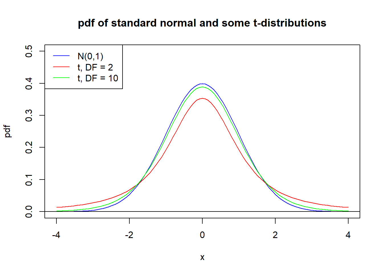
Figure 4.2: Standard normal and two t-distributions.
4.4.3 The one sample \(t\) test - Large sample case
This is a very common test taught in all basic statistics courses. The parameter is a population mean. The alternative hypothesis is one of the following.
- \(H_1: \mu > \mu_0\)
- \(H_1: \mu < \mu_0\)
- \(H_1: \mu \ne \mu_0\);,
where \(\mu_0\) is some fixed number. We assume the null hypothesis \(H_0\) states \(\mu = \mu_0\). In any case, we will look at a sample of values \[ x_1, x_2, \ldots ,x_{n} \] from the population. We assume for now that \(n \geq 30\), which is what we call a large sample case. Some modifications are required for smaller samples. The test statistic will be \[ T = \frac{\bar{x} - \mu_0}{S_x/\sqrt{n}} \] and this will have a \(t_{_{DF = n-1}}\) distribution given that \(H_0\) is true. Given the sample, we would (using e.g. R) compute the observed value, \(T_{_{OBS}}\), and depending on which form of a) b) and c) we have on the alternative hypothesis, a \(P\)-value can be computed. Considering carefully the three cases we find that
- In this case, if \(\bar{x} \leq \mu_0\) we have no evidence for \(H_1\). If \(\bar{x} > \mu_0\), the larger the value on \(\bar{x}\), the stronger the evidence for \(H_1\). A larger value for \(\bar{x}\) corresponds to a larger value for \(T\). Thus the \(P\)-value becomes \(P[T > T_{_{OBS}}]\) computed using a t distribution.
- Here, if \(\bar{x} \geq \mu_0\), we have no evidence for \(H_1\). If \(\bar{x} < \mu_0\), the lower the value for \(\bar{x}\), the stronger the evidence for \(H_1\). This corresponds to a larger negative value for \(T\). So, the \(P\)-value becomes \(P[T < T_{_{OBS}}]\) computed using a t distribution.
- In this case, the further away \(\bar{x}\) is from \(\mu_0\), the stronger the evidence for \(H_1\). This corresponds to a \(T\) value further away from 0. Now the \(P\)-value becomes \[ 2 P[T> |T_{_{OBS}}|] \;. \]
The cases a) and b) are called one-sided or one-tailed alternative hypotheses. Case c) is called two-sided or two-tailed.
Example 4.2 (Quality Control) A machine is supposed to fill bottles with 0.50 liters of mineral water. The content in each individual bottle deviates a little from 0.50, but the producers are happy if the mean \(\mu\) is close to 0.50. On the other hand, if evidence is found that the mean is different from 0.50, the machine must be taken out of production and serviced. For quality control a sample of 30 bottles is taken out to test whether the machine works properly. A reasonable test for this problem is \[ H_0: \mu = 0.50 \ \mbox{vs.} \ H_1: \mu \ne 0.50. \] Suppose the sampling gives \(\bar{x} = 0.505\) and \(S=0.009\). Set \(\alpha = 0.05\). Should \(H_0\) be rejected on basis of these observations? Let us compute the observed value for the statistic, and then find an approximate \(P\)-value. We easily find \[ T_{_{OBS}}= \frac{\bar{x} - 0.50}{{S / \sqrt{n}}} = \frac{0.505 - 0.50}{{0.009 / \sqrt{30}}} = 3.04 \] The \(P\)-value is given by a \(t\) distribution with DF = 29. This is close to a \(N(0, 1)\) distribution and using that as a good approximation we get \[ P = 2 P[ T > 3.04 ] = 2\cdot(1 - P[T \leq 3.04]) = 2\cdot(1 - 0.9988) = 0.0024 \] Assuming the significance level is 0.05, the found \(P\)-value is way below this, and we should reject \(H_0\). We have strong evidence that the machine is not working properly, and it should be taken to service.
4.5 Hypothesis testing with R - one-sample t-test
R of course has a large number of built-in procedures/functions for
testing of statistical hypotheses. Some of them are “stand-alone”
procedures, some are part of larger analyzes. To exemplify how we typically do a stand-alone test, let’s look at the R
version of the one sample \(t\) test. We will look at a practical example. A transportation company in an urban area
has a computer system for planning of delivery routes. In parts of the planning, a mean \(\mu\) for the time to get from
one customer to another must be submitted. The planners are operating with \(\mu = 20\) minutes. New data are available, and one
wants to test whether the new data strongly indicates that the figure \(\mu = 20\) is wrong. This can be formulated as a
test, set up as
\[ H_0: \mu = 20 \ \mbox{vs.} \ H_1: \mu \ne 20\;. \]
The alternative is two-sided. We want significance level \(\alpha = 0.05\). The data file, called Trip_durations.csv
must be loaded into R. We can do that, and look at the first few rows of data. Note again that when reading data into
R, we need to be careful with the data types.
In this case the data columns are separated by “,” and the decimal separator is “.”, so we want the data to be interpreteded as decimal numbers. We can use the function read.csv as below in this case. Again, recall that the file path below should be replaced by the path on your PC.
#the
trips <- read.csv("Data/Trip_durations.csv", dec = ".")

#look at top rows, and a summary of the duration variable:
head(trips)
## Duration Distance
## 1 12.5 2.74
## 2 33.5 13.60
## 3 33.1 10.99
## 4 37.0 10.31
## 5 18.3 4.93
## 6 29.3 8.15## Min. 1st Qu. Median Mean 3rd Qu. Max.
## 9.40 19.50 23.70 24.31 29.32 41.70There are two variables, representing the time duration and distance for \(n = 200\) customer-to-customer trips. We shall later on investigate the relationship between the two variables, but for now we are only concerned with testing the mentioned hypothesis regarding the mean duration \(\mu\). From the summary, we see that the sample mean (\(\bar{x}\)) is 24.31. Obviously this is different from 20, but is the difference significant?
We will use the R function t.test to find the \(P\)-value for the test. This function can be specified to work for many versions of the t-test, here is what we need in this case.
#run and save the test results:
mytest <- t.test(trips$Duration,
                 alternative = "two.sided",
                 mu = 20)
So, we are asking R to run the one-sample t-test, using data in the Duration column of my dataframe, with a two-sided alternative, and \(\mu = 20\) as the null hypothesis. The result is not shown when we do it like this, but is stored in the object mytest. We can then investigate relevant parts of this object, or print the whole content.
## [1] 3.08678e-16## [1] 23.35737 25.26363
## attr(,"conf.level")
## [1] 0.95##
## One Sample t-test
##
## data: trips$Duration
## t = 8.9181, df = 199, p-value = 3.087e-16
## alternative hypothesis: true mean is not equal to 20
## 95 percent confidence interval:
## 23.35737 25.26363
## sample estimates:
## mean of x
## 24.3105It turns out the \(P\)-value is practically 0, corresponding to the \(T_{_{OBS}}= 8.92\) value reported. The extremely low \(P\)-value means we should reject \(H_0\) clearly here. A 95% confidence interval for true mean \(\mu\) is approximately [23.36, 25,26].
To see this result in light of our statistical thinking, consider the following. We observe \(\bar{x} = 24.31\). This is different from 20 as claimed in \(H_0\). However, we will always observe \(\bar{x} \ne 20\) even if \(H_0\) was true, because of natural randomness in the sample. The question again becomes whether the difference is too large to make \(\mu = 20\) a reasonable assumption. So, what is the probability of seeing such data as seen here, given that \(H_0\) is true? This is essentially the \(P\)-value, which is about 0. It means \(\bar{x} = 24.31\) (or further away from 20) is totally improbable if \(\mu = 20\). So we simply don’t believe in \(\mu = 20\). We say that the observed difference is highly significant.
If you look closer at the documentation for the t.test function (use ?t.test at the R prompt) we find that one-sided alternatives \(H_1: \mu > 20\) and \(H_1: \mu < 20\) could be specified as follows, respectively.
mytest2 <- t.test(trips$Duration,
                 alternative = "greater",
                 mu = 20)

mytest3 <- t.test(trips$Duration,
                 alternative = "less",
                 mu = 20)
As expeceted, the \(P-value\) is very close to 0 for the first test, while practically equal to 1 for the other test. So, only in the first of these cases would we reject \(H_0\) in favor of \(H_1\). we can inspect the \(P\)-values as follows.
#make a vector with the p-values
p_values <- c(mytest2$p.value, mytest3$p.value)

#print the values
print(p_values, digits = 3)
## [1] 1.54e-16 1.00e+00Note that R by default here uses scientific notation for the numbers, i.e the first \(P\) value here is
written 1.54e-16 which means
\[ 1.54 \cdot 10^{-16} = 0.000000000000000154\;.\]
There are ways to force R to use either form, but for now, let’s take what we get.
4.6 Binomial test for proportions
We now turn to the binomial test. This is used for testing hypotheses about population proportions in the same context as in section 2.8.2 when we discussed proportion confidence intervals.
Briefly reviewed, we have a population that is divided into two groups, say A and B, and the parameter \(p\) is the proportion of A’s in the whole population. We saw an example where hypotheses about \(p\) appeared in example 4.1 part 3). In general, the null hypothesis take the form \[ H_0: p = p_0 \;, \] where \(p_0\) is some fixed number, while the alternative can be any of the following.
- \(H_1: p > p_0\)
- \(H_1: p < p_0\)
- \(H_1: p \ne p_0\);.
Clearly, the sample estimate \(\hat{p}\) will be a crucial part of the test statistic. For instance, in case a) of the \(H_1\) hypothesis above, only a value \(\hat{p}\) greater than \(p_0\) will make us even consider rejecting \(H_0\). To see how much greater we need to make use of a proper test statistic. We jump right to the following summary of the binomial test.
- Test Statistic: We use \[ Z = \frac{\hat{p} - p_0}{ \sqrt{\frac{p_0(1-p_0)}{n} }} \] as the test statistic.
- Null Distribution: If the sample size is large enough, so that \(n p_0(1 - p_0) > 5\) we can use the \(N(0,1)\) distribution for \(Z\) as an acceptable approximation.
In this description, we use the terminology null distribution. This is short for the distribution of the test statistic, given that \(H_0\) is true. We will use this terminology in the following.
Example 4.3 Let us return to example 4.1 c), where the parametric form of the hypotheses can be written \[ H_0: p = 0.13 \ \mbox{vs.} \ H_1: p > 0.13 \;. \]
Recalling the example as it evolved, we had \(\hat{p} = 0.16\) from a sample of size \(n = 300\), and this was said not to provide sufficient evidence for \(H_1\). Let us now see why. The test statistic is \(Z\) as defined above. Clearly, a larger value for \(\hat{p}\) constitutes stronger evidence for \(H_1\). That corresponds to a larger value for \(Z\). So to say that \(Z\) is more critical than \(Z_{_{OBS}}\) in this case, means \(Z > Z_{_{OBS}}\). Okay, so what is \(Z_{_{OBS}}\) in this case? Just insert values for \(\hat{p}\) and \(n\) to obtain \[ Z_{_{OBS}}= \frac{0.16 - 0.13}{ \sqrt{\frac{0.13(1-0.13)}{300} }} = 1.55 \;.\] Now, let us find the \(P\) value. Recall, this is the probability of a more critical value for the test statistic than what was observed - given \(H_0\) true, i.e. in this case \[ P = P[Z > Z_{_{OBS}}] = P[Z > 1.55] = 1 - P[Z \leq 1.55] = 1 - 0.9394 = 0.0606 \;. \] The \(P\)-value is low, but not low enough to give what we would call hard evidence for \(H_1\). More formally, assuming we use the level of significance \(\alpha = 0.05\), we see that we can not reject \(H_0\) with the given observation of \(\hat{p}\) at 0.16. In this case, we need to keep the null hypothesis. In practice, it means that there is no convincing evidence that the proportion of customers who actually buy things has increased beyond 0.13.
4.6.1 Binomial test using R.
R offers the function binom.test for performing a binomial test. Most often, our raw data will be a (long)
vector with two values (say A, B or 0, 1) and we have a hypothesis about the true proportion of (say) A’s or 1’s.
We will say here that we call \(p\) the true proportion of “successes” in the population.
We need to be clear about what constitutes a “success” in our data. To use the binom.test we usually
need to know the number of observed successes, and the number of observed failures. This can be easily obtained using the table function. We give a vector with counts of successes and failures to binom.test along with a specification of alternative form, and the value of \(p_0\). We better look at a concrete example.
Example 4.4 Suppose employees in a certain industry is asked whether they prefer
- A: 10% increase and keeping the current work week.
- B: Keeping the current salary but having a 10% shorter working week.
Suppose a large survey in Sweden revealed that the proportion who prefer alternative A is \(p_s = 0.80\). Based on a sample of 200 Norwegian workers in the same industry, one wants to test whether the proportion \(p\) preferring alternative A is different from 0.80. So, the hypotheses are \[ H_0: p = 0.80 \ \mbox{vs.} \ H_1: p \ne 0.80\;. \]
The data in this case is simply a variable called raise with values 0 and 1, where 1 means the respondent prefer alternative A, while 0 means
preference for alternative B. The encoding with 0, 1 is completely arbitrary, any two values or strings would work.
To run the binomial test we need (of course) to load the data, to find the count of successes and failures (carefully!)
and then feed this to the binom.test function.
##   raise
## 1     1
## 2     1
## 3     0
## 4     0
## 5     1
## 6     0
We see the first few 0’s and 1’s. Note that 1 means “success” in the setting of this example.
##
##   0   1
##  74 126
So we get 74 failures and 126 successes. We need to reverse the order of the counts vector before giving it to the binom.dist function. There are various ways to do that, but below is the most straightforward, simply
indexing the vector by 2:1 or identically by c(2, 1) . Then we do the test.
##
##   1   0
## 126 74##
## Exact binomial test
##
## data: counts
## number of successes = 126, number of trials = 200, p-value = 2.49e-08
## alternative hypothesis: true probability of success is not equal to 0.8
## 95 percent confidence interval:
## 0.5590535 0.6970302
## sample estimates:
## probability of success
## 0.63So, as we see, the count of 126 successes in 200 trials give the estimate \(\hat{p} = 0.63\) for \(p\). In terms of the test we performed, the \(P\)-value is again extremely low, so at a significance level of 0.05 we would clearly reject \(H_0\) here and conclude that the proportion in Norway is very likely lower than 0.80 (i.e. 80%).
4.7 Two-sample t-test (Independent samples t-test)
The final of the basic tests we consider in this chapter is the two-sample t test. This is what we would use in a situation like example 4.1 a). There, two separate mean values are compared. In this case, the means are square meter prices for sold houses in two months. It is very natural to compare such means, and to want to test whether one is larger than the other. You will often see this test called also an “independent samples t test”.
In a general setup for the two-sample t test, we consider two populations (or systems) A and B. We are interested in the means for a variable in the two populations (e.g. the populations could be houses sold in April and in May, the variable could be the square meter prices for each sold house). In general notation, we write \(\mu_x, \mu_y\) for the two means from population A and B respectively. The null hypothesis is almost always on the form \[ H_0: \mu_x = \mu_y \;, \] while the alternative can be any of the following.
- \(H_1: \mu_x > \mu_y\)
- \(H_1: \mu_x < \mu_y\)
- \(H_1: \mu_x \ne \mu_y\);.
To test the hypotheses, we then need samples from the two populations, \[ x_1, x_2, \ldots ,x_{n_x}, \quad y_1, y_2, \ldots ,y_{n_y} \;, \] and compare the sample means \(\bar{x}\) and \(\bar{y}\). Obviously, a “large” difference in the right direction would lead us to believe in the alternative hypothesis, e.g. \(\bar{x} > \bar{y}\) would point in the direction of \(H_1\) in case of alternatives a) and c). (Not in case b) - why?) But what is a “large” difference? Once again, we need to consider a test statistic and a null distribution to answer this. The details of this is summarized as follows.
- Test Statistic We use \[ T = \frac{\bar{x} - \bar{y} }{ \sqrt{\frac{S_x^2}{n_x} + \frac{S_y^2}{n_y}}} \] as the test statistic. Here, \(S_x^2, S_y^2\) are the sample variances, and \(n_x, n_y\) are the sample sizes.
- Null Distribution If the samples are both larger than 30, a \(t\) distribution is used for the null distribution. The degrees of freedom result from a complicated expression, which we will not need. For hand calculations, a \(N(0, 1)\) distribution is an acceptable approximation. Smaller samples will require some modifications.
Example 4.5 (Comparing Flat Prices) We return to our initial example 4.1 a) about mean house prices. In the final case of that example, summary data for a sample of prices in April and May was given. The data is reviewed inn table 4.1. We can use these data to perform a two-sample t-test for a possible increase in mean price levels for April and May. Let \(\mu _x, \mu_y\) denote the total mean square meter prices for April and May. The hypotheses would be \[ H_0: \mu_x = \mu_y \ \mbox{vs.} \ H_1: \mu_x < \mu_y\;. \]
| Month | mean | standard-deviation | sample-size |
|---|---|---|---|
| April | \(\bar{x}=19800\) | \(S_x=350\) | \(n_x=300\) |
| May | \(\bar{y}=20100\) | \(S_y=410\) | \(n_y=200\) |
We note that \(\bar{x} < \bar{y}\), so that the data points to the alternative hypothesis. It is not clear at the moment if this is strong evidence for \(H_1\). We need to find the value for \(T_{_{OBS}}\), and then the \(P\)-value, based on the \(N(0,1)\) distribution which in this case is a very good approximation (large samples). We note that the critical direction for \(T\) values is in the negative direction. It is an easy matter to find \[ T_{_{OBS}}= \frac{19800 - 20100 }{ \sqrt{\frac{350^2}{300} + \frac{410^2}{200}}} = -8.49 \;. \] The \(P\)-value is the probability of an even more critical value. Using standard normal distribution, we know that practically speaking, \[ P[T < -8.49] = 0 \;. \] So the \(P\)-value is almost 0, and we reject \(H_0\) in favor of \(H_1\). The sample shows overwhelming evidence that the mean price was higher in May than in April.
Now, let us turn to how a two-sample t test can be done with R. First a note on how the data should look for such a test. We should have our variable of interest \(x\) (e.g. square meter prices) and the variable defining groups in a dataframe, so the structure of data should be something like this:
##    x G
## 1 34 A
## 2 31 A
## 3 31 B
## 4 33 B
## 5 41 A
## 6 41 A
## 7 34 B
## 8 34 B
with possibly many other variables in addition. So here, the variable \(G\) is a grouping variable that
defines which groups of \(x\) values we want to compare. To make this specification in R, we use an R formula which in this case is the expression x ~ G. So, in general this means we will study x depending on the values of G. The general syntax will then be something like
t.test(DF$x ~ DF$G, ...) or maybe more aesthetically, with(DF, t.test(x ~ G, ...)). Those two expressions do exactly the same. The variable \(G\) will in general divide the data into groups of unequal size.
Example 4.6 (Post-operation recovery times) Suppose two hospitals in Norway perform a routine surgical procedure in slightly different ways. After the operation, patients must stay off work/school for a variable number of days. With sample data from the two hospitals, one may run a two-sample t-test to compare the mean duration of post-operative inactivity for the patients. Suppose the hospitals are labeled A and B. If we denote by \(\mu_A, \mu_B\) the two means, we would be interested in testing \[ H_0: \mu_A = \mu_B \ \mbox{vs.} \ H_1: \mu_A \ne \mu_B\;. \]
As usual we must read in the data, then we can take a look at the structure.
#read the data
hospitaldata <- read.csv2("Data/Hospital_durations.csv")

#look at top rows
head(hospitaldata)
## Hospital Inactive
## 1 A 15
## 2 B 12
## 3 A 14
## 4 B 15
## 5 A 12
## 6 B 14So, we see the variables Hospital (grouping variable) and Inactive which is the number of days of inactivity, this is our variable of interest. Now, let us do the t-test comparing the means of Inactive between the two hospitals.
##
##  Welch Two Sample t-test
##
## data:  Inactive by Hospital
## t = -2.7157, df = 97.863, p-value = 0.00782
## alternative hypothesis: true difference in means between group A and group B is not equal to 0
## 95 percent confidence interval:
##  -1.8692111 -0.2907889
## sample estimates:
## mean in group A mean in group B
##           14.02           15.10
We see that the mean in group A is a little more than a day lower than group B. Considering the \(P\)-value at 0.008, this is significant even at the 0.01 level.
4.8 Small sample t-tests
Without going into much detail, let us briefly comment on the issues that need to be taken into account for t-tests when our sample is of size less than 30, i.e. what is called the small sample case. The important thing to remember in this case, is that we need to impose certain assumptions on the distribution of our data. Looking for instance at the one-sample t-test, we base our decision on a sample \[ x_1, x_2, \ldots ,x_{n} \] of values, recorded from some variable \(x\) describing a population. When \(n < 30\) our results from a one-sample t-test are only valid if the \(x\) variable we observe is approximately normally distributed. Based on how our \(n\) sample values are distributed, we can make a judgement of the distribution of \(x\). If evidence is found that \(x\) is not normally distributed, we can not rely on results of t-tests. Regarding a two-sample test, this assumption of normal data must be imposed on data in both groups, if both samples are small.
4.8.1 Testing normality of data
In connection with the assumption about normal distribution of data above, there are ways in R to test such assumption. There is a visual method called a normal QQ-plot, where a given vector \(x\) of observations is plotted against an idealized sample from a normal distribution. If \(x\) is sampled from (close to) a normal distribution, the plot should show data points approximately on a straight line. To show this, we can make a simulation, where we simulate normal data \(x\) and non-normal data \(y\), and then look at the qq-plots as produced by R.
Example 4.7 (Simulation: normal and non-normal data) So, we use R to draw from a normal distribution, and then from a \(t\) distribution with DF = 2, and see how the plots come out. We sample 150
values for each. The relevant function in R is qqnorm.
#set seed for random generator
set.seed(43)
#sample two vectors.
x <- rnorm(150, mean = 20, sd = 2)
y <- rt(150, df = 2)
par(mfrow = c(1,2))
qqnorm(x, main = "Data are normal")
qqnorm(y, main = "Data are not normal")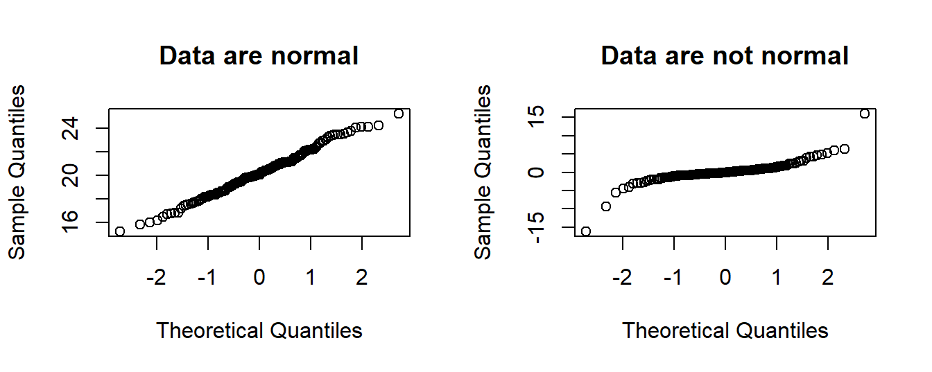
We see that the plot on the right have some striking deviations away from the straight line, indicating that these data are not normally distributed. In the left plot, there are only small deviations.
In addition to these plots, we can make a formal hypothesis test, called “Shapiro test”. Here \(H_0\) states that data (a vector) are normal, while the alternative is “not normal”. A small P-value is an indication of non-normality, as this means we would reject the \(H_0\). Let’s see for our \(x\) and \(y\) above:
##
##  Shapiro-Wilk normality test
##
## data:  x
## W = 0.9943, p-value = 0.8241##
## Shapiro-Wilk normality test
##
## data: y
## W = 0.74861, p-value = 9.79e-15Here \(W\) is a particular test statistic, while we see the P-values makes us keep \(H_0\) for \(x\), and reject \(H_0\) for \(y\). So that’s the same conclusion as indicated by the QQ plots.