Chapter 2 Random variables - inferential statistics.
In this chapter we quickly review some facts about random variables, and introduce the concept of inferential statisics with the most basic confidence intervals as examples.
2.1 Random variables
Let us review some core properties of random variables and probability distributions. We will focus exclusively on basic ideas that we will need in the following chapters. We start with an informal definition of a random variable. Essentially, a random variable is any quantity \(X\) for which there is more than one possible value. Random variables are also called stochastic variables. Associated with possible values is a probability distribution. In general, there are two types of random variables.
- Discrete A random variable \(X\) is discrete if there is a distinct set of values \(x_i\) that \(X\) can have.
- Continuous A random variable \(X\) is continuous if \(X\) can have any value in an interval. This means that for any two values \(x_1, x_2\) there will be values between \(x_1, x_2\) that \(X\) can have.
We’ll do some examples, but first note that the distinction here is essentially the same as what we did in section 1.3.1 for variables in a data set. What we call “variables” in a data set is almost always just observed values of a corresponding random variable.
Before looking at some examples, let us just recall the general notation for probabilities, where \(P[\cdots]\) means the probability of some outcome relating to a random variable. So if \(X\) is some random variable, then \(P[X=3]\) is the probability that \(X=3\), \(P[2 \leq X \leq 10]\) is the probability that \(X\) comes between 2 and 10 and so on.
Example 2.1 (Discrete random variable) If we let \(X\) denote the number of driveable cars in a randomly selected family/household, it is clearly discrete. Possible values are \(X = 0, 1, 2, 3, \ldots\). A probability distribution would have to be estimated from data. In Norway it could possibly be something like \[ P[X = 0] = 0.25, \quad P[X = 1] = 0.50, \quad P[X=2] = 0.20, \quad P[X=3] = 0.04, \ldots\] where the remaining probabilities are ignorable. Note that since \(X\) is discrete, it makes sense to assign positive probabilities to single outcomes like \(P[X=1]\). Also note that \(X\) can be 1 or 2 but no intermediate value for \(X\) is possible.
Example 2.2 (Continuous random variable) Now, suppose \(X\) denotes the amount of fuel consumed by a large fleet of commercial airplanes during a month of operation. Typically it would be many thousands of tons. If any two values are possible, then also any value in between must be possible. So we should consider \(X\) to be continuous. In this case it is not possible to assign a positive probability to any particular value. We will instead speak of the probability that \(X\) takes values in intervals, i.e. for given numbers \(a, b\) we consider probabilities \[ P[X \leq a] \ \mbox{and} \ P[a \leq X \leq b] \] To accommodate this we use a probability density function, i.e. a curve such that the area below the curve between \(a\) and \(b\) equals \(P[a \leq X \leq b]\). The idea is illustrated in figure 2.1 below, where the curve represents the probability distribution of \(X\), and \(a, b\) are some numbers in a relevant range. Here \(f(x)\) is the probability density function. We do not need to bother with specific numbers at this point. Of course there are ways to specifically compute such probabilities given the function \(f\) and the values \(a, b\).

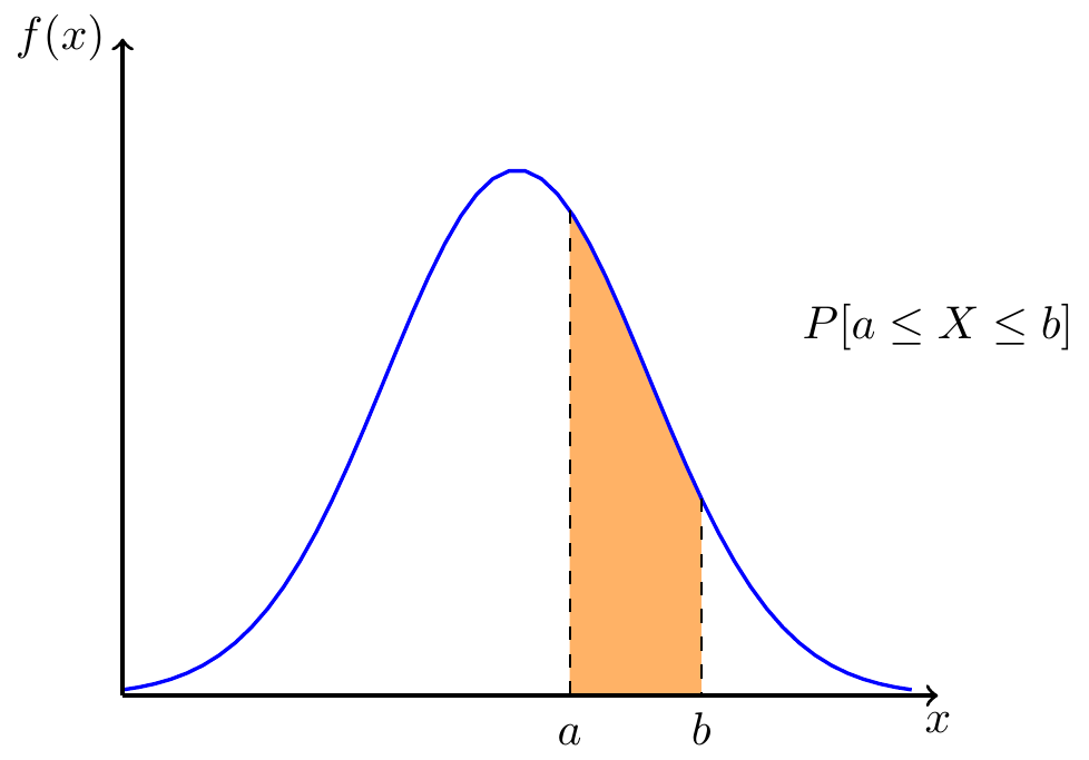
Figure 2.1: Probability densities
2.2 Mean and standard deviation.
For a given random variable \(X\) (and its distribution), there are two parameters of fundamental interest. The theoretical mean of \(X\) is denoted by the greek letter \(\mu\). It is also called the expected value of \(X\), written \(\mbox{E}{[X]}\). We interchangeably use both notations and stress that \[ \mu = \mbox{E}{[X]} \;. \] We will not review the particular definitions of the mean here. It suffices to have the intuitive understanding that if we observe a long series of values (a sample) \[ x_1, x_2, \ldots ,x_{n} \] for a random variable \(X\), the average value \(\bar{x}\) will be “close” to \(\mu\). We will make this more precise in a short while, but the case is essentially that as \(n\) grows larger, \(\bar{x}\) approaches the theoretical mean value \(\mu\). For this reason it makes sense to estimate the value \(\mu\) with the sample mean \(\bar{x}\). Sometimes we shall operate with several random variables \(X, Y, \ldots\) at a time. To emphasize which means belong to which variables, we will then typically write \[ \mu_x = \mbox{E}{[X]}, \quad \mu_y = \mbox{E}{[Y]}, \cdots \]
The second parameter of fundamental importance for a random variable is the theoretical standard deviation. This is commonly denoted by the greek letter \(\sigma\), and is also commonly denoted by \(\mbox{Sd}{[X]}\). We use both notations and often write \[ \sigma = \mbox{Sd}{[X]} \] to make it very clear what we are talking about. The theoretical variance is simply the square of the standard deviation, and it is then written \(\sigma^2\) or \(\mbox{Var}{[X]}\). The theoretical standard deviation is strongly related to the sample standard deviation \(S\) discussed earlier. Indeed, if we have a sample \[ x_1, x_2, \ldots ,x_{n} \] of observed values for a random variable, then the idea is that \(S\) is “close” to \(\sigma\) in the same sense as for the mean values above. When sample size \(n\) grows, \(S\) will approach \(\sigma\). Thus we will estimate the parameter \(\sigma\) with \(S\).
2.3 The normal distribution
The normal distributions are central to basic statistics. Most readers presumably have some familiarity with this family of distribution. Any text on basic statistics will have a chapter devoted to normal distributions, so here, we review quickly the most important features. If \(\mu, \sigma\) are given values for a mean and a standard deviation, there is a particular normal distribution with these parameter values. The shape of the normal probability density function is pretty much like the one seen above. The general normal density function is given by the expression \[ f(x) = \frac{1}{\sqrt{2 \pi} \sigma} e^{-\frac{(x - \mu)^2}{2\sigma^2}} \;. \] For those who now start to worry about the mathematics, be calm — we are not going to work on this expression at all, it is just included for the sake of completeness. Drawing out two particular normal curves gives an idea of the role of the parameters \(\mu\) and \(\sigma\). In figure 2.2 we see normal distributions. The means are \(\mu = 3\) and \(\mu = 5\) respectively. Note that these values are the \(x\)-coordinate of the top point of the curve. Secondly, the standard deviations of the curves are \(\sigma = 1\) and \(\sigma = 2\) respectively. Note how the larger \(\sigma\) gives a more spread-out distribution for the values of the random variable. Further note that for both normal distributions, much of the probability lies within \(\pm 2\sigma\) from the mean \(\mu\). In fact one can prove that for any normal variable \(X\), the probability that \(X\) is between \(\mu \pm 2\sigma\) is 95.5%. Taking \(\pm 3\sigma\) leaves a probability of 99.7% in the interval. So, knowing \(\mu\) and \(\sigma\) gives us some intervals where \(X\) will very likely have its value. As a small exercise, check for the two normal distributions in figure 2.2: Where is the interval \(\mu \pm 2\sigma\)? Note how little of the probability remains outside of the interval. Do the same with \(3 \sigma\) and note that virtually 0 probability is outside of the interval. These interval properties are the theoretical counterparts of the empirical rule outlined in section 1.4.2.
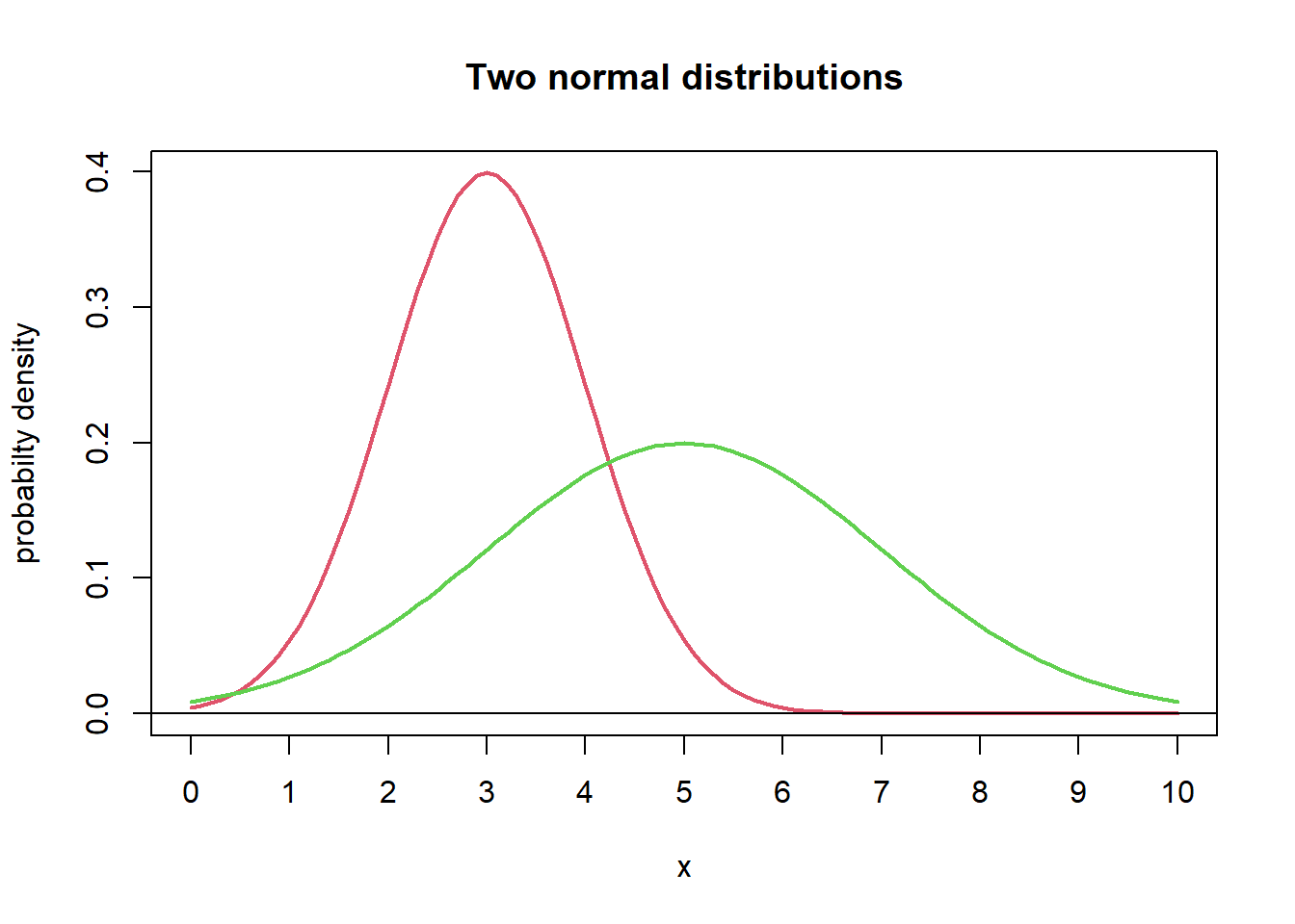
Figure 2.2: Two normal distributions
We will write \[ X \sim N(\mu, \sigma) \] to express that \(X\) is a normally distributed random variable with the given mean and standard deviation. So in figure 2.2 we see the distribution of a \(N(3,1)\) variable, and a \(N(5,2)\) variable.
2.3.1 The standard normal distribution
If \(\mu = 0\) and \(\sigma = 1\) we call the resulting normal distribution the standard normal distribution. It is customary to write \(Z\) for a standard normal variable. Then we know that \[ \mbox{E}{[Z]} = \mu = 0, \quad \mbox{Sd}{[Z]} = \sigma = 1 \;. \] In line with the above, we will see a curve with almost all probability assigned to the interval between -3 and 3. See figure 2.3. In correspondence with the notation introduced above, we can write \(Z \sim N(0,1)\).
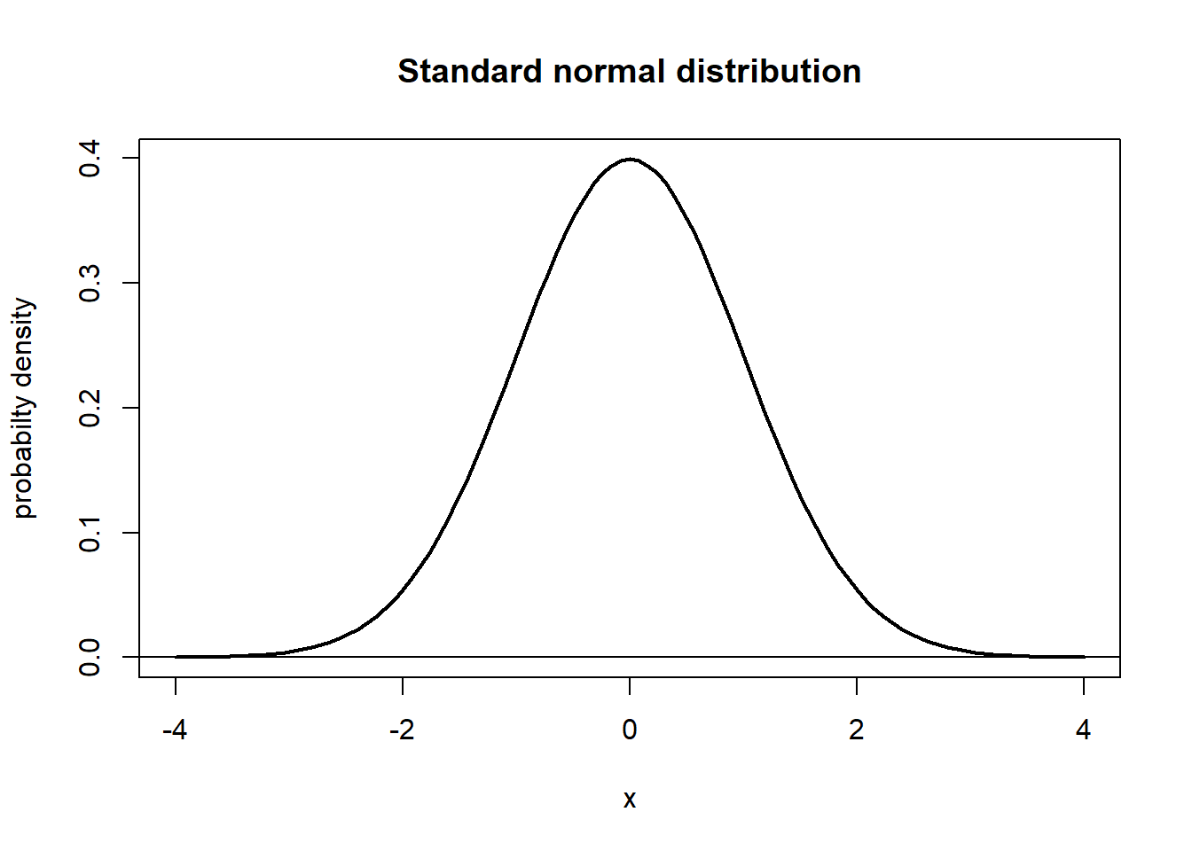
Figure 2.3: Standard normal distribution
The process of standardization makes it possible to transform any statement or question about a general normal variable \(X\) into a corresponding question about a standard normal variable \(Z\). The standardization of \(X\) is the result of subtracting the mean \(\mu\) and then dividing by the standard deviation \(\sigma\). So, for a general \(X \sim N(\mu,\sigma)\), we write \[\begin{equation} Z = \frac{X - \mu}{\sigma}\;. \tag{2.1} \end{equation}\] Now, \(Z \sim N(0,1)\). Assuming for the moment that we know how to find probabilities for the standard normal distribution, let us see an example of how the standardization works.
Example 2.3 (Standardization) Suppose \(X \sim N(100, 20)\). Find the standardized versions of the following.
- \(P[X \leq 140] =\)?
- \(P[X \geq 70] =\)?
- For what value \(b\) is \(P[X \leq b] = 0.90\)?
Preliminary solution:
- Standardize the statement \(X \leq 140\) as follows. \[\begin{eqnarray*} X \leq 140 \Rightarrow X - \mu \leq 140 - \mu \\ \Rightarrow \frac{X - \mu}{\sigma} \leq \frac{140 - \mu}{\sigma} \\ \Rightarrow Z \leq \frac{140 - 100}{20} = 2 \end{eqnarray*}\] i.e. the original probability equals \(P[Z \leq 2]\).
- Same procedure leads to \(P[X \geq 70] = P[Z \geq -1.5]\)
- Compute as follows: \[\begin{eqnarray*} X \leq b \Rightarrow X - \mu \leq b - \mu \\ \Rightarrow \frac{X - \mu}{\sigma} \leq \frac{b - \mu}{\sigma} \\ \Rightarrow Z \leq \frac{b - \mu}{\sigma} \end{eqnarray*}\] Suppose you knew somehow that \(P[Z \leq c] = 0.90\) implies \(c = 1.28\). Then by the above, \[ \frac{b - \mu}{\sigma} = c \Rightarrow b = \mu + c \sigma = 100 + 1.28 \cdot 20 = 125.6 \;,\] i.e. we should take \(b=125.7\) to get \(P[X \leq b] = 0.90\).
The solution in part 1 of example 2.3 is visualized in figure 2.4 Note how the distribution shape is unchanged, while the underlying scale changes.
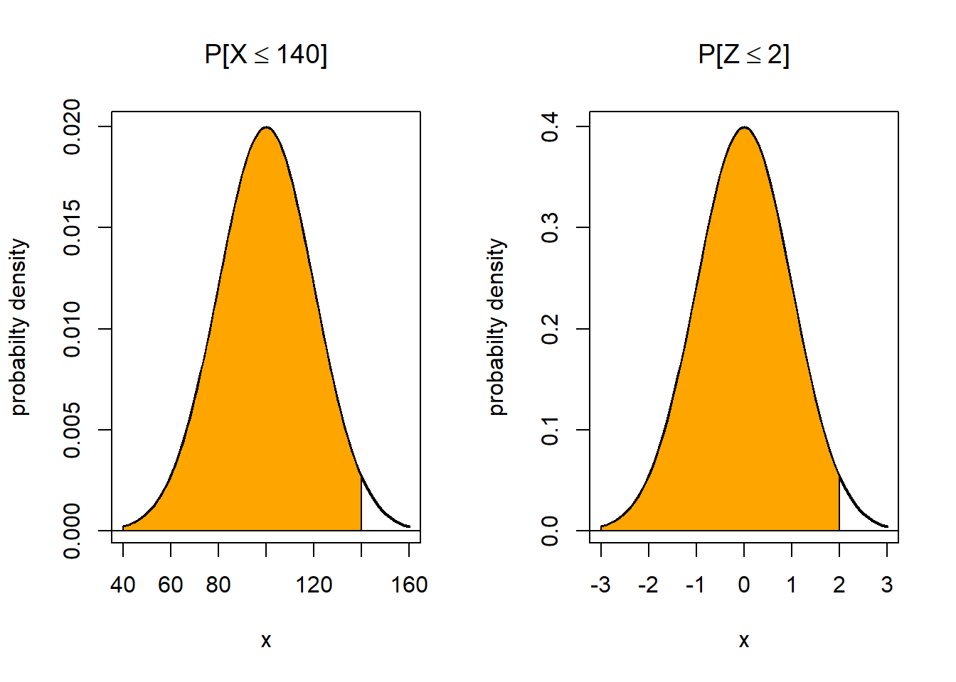
Figure 2.4: The effect of standardization
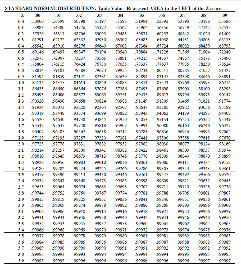
Following up on example 2.3, we now need to know how to address the questions relating to the standard normal variable. The “manual” way is to use a probability table for the standard normal distribution. An example of such a table is included in section 2.8.3 at the end of this chapter.
The table provides values for \(P[Z \leq z]\) for \(z\) values \[ 0.00, 0.01, 0.02, \ldots, 3.99\;. \] To find e.g. \(P[Z \leq 1.34]\) we first find the row with \(z = 1.3\) in the leftmost position. Then we find the column with 0.04 in the top position. The number in that row/column is the probability we want: \[ P[Z \leq 1.34] = 0.9099\;. \] All other relevant probabilities for a standard normal variable can be derived from the limited set provided by the table. The reader should make sure to understand that symmetry of the \(N(0,1 )\) distribution and the law of complement implies that we may do the following type of computations.
- By the law of complement, \(P[Z \geq 1.22] = 1- P[Z \leq 1.22] = 1 - 0.8888 = 0.1112\).
- By symmetry, \(P[Z \geq -1.33] = P[Z \leq 1.33] = 0.9082\).
- By combination, \(P[Z \leq -2.4] = P[Z \geq 2.4] = 1 - P[Z \leq 2.4] = 1 - 0.9918 = 0.0082\;.\)
(For any event \(A\) with a probability \(P(A)\) let \(\overline{A}\) denote the event that \(A\) does not occur. I.e. \(\overline{A}\) is the opposite of A. Then the law of complement states that \(P(\overline{A}) = 1 - P(A)\).))
Relating to the question in example 2.3 part 3, we were led to look for a value \(c\) such that \[ P[Z \leq c] = 0.90\;. \] To find \(c\) we need to use the standard normal table in “reverse”. We try to locate the probability that is closest to 0.90, and then find the corresponding \(z\) value. You will find that \(z = 1.28\) is a good choice, because \[ P[Z \leq 1.28] = 0.8997\;\] according to the table. We could look for further decimals of precision, but that is not important for our purposes.
Example 2.4 (Resolving example) We now complete the calculations for the example 2.3.
- By checking the normal table we find \[ P[X \leq 140] = P[Z \leq 2] = 0.9772\;. \]
- We find by symmetry \[ P[X \geq 70] = P[Z \geq -1.5] = P[Z \leq 1.5] = 0.9332\;. \]
- We found above that \(P[Z \leq c] = 0.90\) implies \(c = 1.28\). Following the computations in example 2.3 part 3, we get to the answer \(b = 125.6\).
2.3.2 Cut-off points for the standard normal distribution
We saw above that given the probability \(p = 0.90\), we should take \(z = 1.28\) to obtain \[ P[Z \leq z] = p = 0.90\;. \] By symmetry, we get \[ P[Z \geq z] = 0.10 \] The value \(z = 1.28\) is called the 0.10 or 10 percent cut-off point of the (standard) normal distribution. It is commonly labeled \(z_{0.10}\). We generalize this for any small probability \(r\) and define the \(r\)-cut-off point \(z_r\) by \[ P[Z \geq z_r ] = r \ \mbox{or equivalently} \ P[Z \leq z_r ] = 1 - r \;.\] The reader should verify from the normal table that \[\begin{equation} z_{0.05} = 1.64, \quad z_{0.025} = 1.96, \quad z_{0.01} = 2.33 \;. \tag{2.2} \end{equation}\] We will see these cut-off values again and again through the following chapters.
2.5 Practical use of random variables.
Random variables are typically used for modelling and describing uncertainty in real world situations, for example within economics or logistics. For example, the future cost of producing a unit of some commodity is usually subject to uncertain factors. Therefore, it can be described as a random variable \(W\). In general, to make such models at all useful, we need to know something about the probability distribution of the variables. Is it discrete or continuous? What is the mean \(\mu\) and standard deviation \(\sigma\)? Can we actually assume with confidence that the distribution is normal? Often, in practice, we have to live with approximate answers to such questions. We need to estimate \(\mu\) and \(\sigma\), and we need to look into the question of the actual probability distribution. This is sometimes complicated, but one “golden rule” can be applied:
If a variable \(W\) is mainly affected by many different random factors, the distribution of \(W\) will tend to be close to normal.
So, very informally, if we have a variable \(W\) which we understand to be affected by many factors, none of which are clearly dominant, we should suspect a close-to-normal distribution. Examples are: \(W\) is the earnings of Mitsubishi Motor Corporation for the next year, or \(W\) is the average temperature in Molde for the coming January month. Note: Both variables can be important for planning purposes, estimates based on historical data plus additional forecasts may help us to get approximate values for \(\mu, \sigma\). Note also that we just learned in the previous section how to answer important probabilistic questions about \(W\), if we say that the distribution is normal, and we know \(\mu, \sigma\). For example we could figure out that with probability 0.95, the average temperature will be above -1.3\(^\circ\)C.
2.6 Joint distribution, correlation coefficient
In most interesting uses of random variables, we are interested in possible relationships between them. For the purposes of this course, we can discuss this topic with the use of covariances and correlations. We discussed sample covariance and correlation in chapter 1. Of course there are theoretical counterparts to these descriptive measures. So, suppose \(X, Y\) are variables with some probability distribution. We then define the covariance between \(X\) and \(Y\) as \[ \sigma_{xy}= \mbox{Cov}{(X, Y)} = \mbox{E}{[(X - \mu_x)(Y - \mu_y)]}\;. \] Here \(\mu_x, \mu_y\) are the means for the two variables. Intuitively, the covariance is positive in a situation where cases of \(X > \mu_x\) tend to come along with \(Y > \mu_y\), and \(X < \mu_x\) tend to come along with \(Y < \mu_y\). For example, if \(X\) is the number of customers and \(Y\) is the turnover in a grocery store on a given day, we should have \(\sigma_{xy} > 0\). The reader can surely provide an example of variables with negative covariance.
More useful than the covariance is the correlation coefficient \(\rho_{xy}\), which is simply defined as \[ \rho_{xy} = \frac{\sigma_{xy}}{\sigma_x \cdot \sigma_y}\;, \] where now \(\sigma_x, \sigma_y\) are the standard deviations of the variables. In the same way as for the sample correlation, we have \(\rho_{xy}\) always between -1 and 1. A correlation of -1 or +1 means the variables are completely linearly dependent, so the value of \(X\) determines the value of \(Y\) with perfection. This is unusual, and rather uninteresting from a probabilistic perspective. The opposite situation is when \(\rho_{xy} = 0\). This means that there is no (linear) relationship between \(X\) and \(Y\). In this case, knowing \(X\) does not tell anything about the value of \(Y\).
2.7 Linear combinations of random variables
When we work with models involving random variables, we very often encounter a situation where some variable is a linear combination of other variables. In the simplest case this means that we have a variable \(W\) of interest, which can be expressed as \[ W = aX + bY \] where \(X\) and \(Y\) are some other variables. The topic we will be discussing, is to what extent knowledge of \(X, Y\) can be converted to knowledge about \(W\). Let’s motivate with an example.
Example 2.5 Suppose a factory produces some commodity, and to produce one unit of the commodity, they use 3 units of raw material A, and 4 units of material B. If future cost of the materials are uncertain, they can be modeled by random variables \(X\) and \(Y\). The total raw material cost per unit is then a new variable, \[ W = 3X + 4Y\;.\] How is the mean and standard deviation of \(W\) related to those of \(X\) and \(Y\)? Can we say something about the distribution of \(W\) given that of \(X\) and \(Y\)? Answers to these questions follow.
So let’s assume we have a general linear combination like \[ W = aX + bY\;, \] and let \(\mu_x = \mbox{E}{[X]}, \: \sigma_x^2 = \mbox{Var}{[X]}\), \(\mu_y = \mbox{E}{[Y]}, \: \sigma_y^2 = \mbox{Var}{[Y]}\). Also let \(\rho_{xy}\) be the correlation coefficient. In general we then have \[ \mbox{E}{[W]} = \mu_W = a\mu_x + b \mu_y\;. \] So, the expected value for \(W\) is just the same combination of the individual expected values.
What about the variance for \(W\)? This is just slightly more complicated. First, let us consider the case that \(X\) and \(Y\) are uncorrelated, \(\rho_{xy} = 0\). In that case, we get \[ \mbox{Var}{[W]} = \sigma_w^2 = a^2 \sigma_x^2 + b^2 \sigma_y^2 \;. \] So, the variance of \(W\) is a linear combination of the variances, with \(a^2, b^2\) as weights.
What happens to this when \(\rho_{xy} \ne 0\)? We get the more general formula \[\begin{equation} \sigma_w^2 = a^2 \sigma_x^2 + b^2 \sigma_y^2 + 2 ab \sigma_x \sigma_y \rho_{xy} \;. \tag{2.3} \end{equation}\] Note that these formulas are valid regardless of the distribution of \(X\) and \(Y\). They always give the right expected value and variance.
In one case, we get an even more useful result. This is when \(X\) and \(Y\) are both normally distributed. In that case one can show that also \(W\) has a normal distribution. 1
The main point of all this is: if \(W\) has a normal distribution, we actually know how to compute relevant probabilities and related quantities, like in example 2.3.
Example 2.6 (Resolving example) We continue from example 2.5. Let us now assume that we have some model for the mean and variance of the costs \(X, Y\), namely we assume \[ \mu_x = 200, \ \mu_y = 90, \ \sigma_x = 20, \ \sigma_y = 10\;. \] Moreover, let’s assume the costs are positively correlated, with correlation \(\rho_{xy} = 0.40\). Finally, suppose both cost variables are normally distributed.
We can answer the following questions:
- What is the mean and standard deviation of the total raw material cost?
- What is the 5% worst-case scenario value for the cost? (I.e. determine a value \(b\) such that the cost \(W\) is above \(b\) with probability 0.05.)
For the first question, we just employ the formulas above, so the mean cost becomes \[ \mu_W = 3\mu_x + 4 \mu_y = 3\cdot 200 + 4\cdot 90 = 960\;\] The variance of the cost is given by the formula (2.3). Note carefully that we need to calculate \(\sigma_x^2, \sigma_y^2\) to get the variances. The numbers given are standard deviations. That said, we move on to calculate \[\begin{align*} \sigma_w^2 & = a^2 \sigma_x^2 + b^2 \sigma_y^2 + 2 ab \sigma_x \sigma_y \rho_{xy} \\ & = 3^2 \cdot20^2 + 4^2 \cdot 10^2 + 2 \cdot 3 \cdot 4 \cdot 20 \cdot 10 \cdot 0.40 \\ & = 7120\;. \end{align*}\] So, to get the standard deviation for the total raw material cost, we take \[ \sigma_w = \sqrt{7120} = 84.4\;. \] So with these figures, we can answer the second question. Since \(X, Y\) are normal, we see that \(W\) is also normal, and we now have the parameters for the distribution, \(\mu_w = 960, \sigma_w = 84.4\). We are looking for \(b\) such that \[ P[W > b] = 0.05 \;, \] which is the same as \[ P[W \leq b] = 0.95\; . \] Following the same lines as in example 2.3, part 3, we find after standardization that \[ b = \mu_w + z_{0.05} \cdot \sigma_w = 960 + 1.645\cdot 84.4 = 1098.8\;. \] Approximately, the 5% worst-case value for the cost is 1100. This means, there is only a small risk for the cost to exceed this value. Such calculations are typically included in more complex risk-management plans in business and industry. Owners and management obviously want to control the risk in the total operations of the company.
We conclude this section with a couple of related topics. A special case is when a variable is only a multiple of one other variable, i.e. \[ W = aX\;,\] and \(\mu_x, \sigma_x\) is known. Then it follows from the formulas above, that \[ \mu_W = a \mu_x, \quad \sigma_w = a \sigma_x\;.\] So, for example, if \(X\) is the future price of a share, where you assume \(\mu_x = 75, \sigma_x = 5\), and you own 100 of these shares, your whole investment will be worth \[W = 100X\] with expected value \(\mu_w = 100 \mu_x = 7500\) and standard deviation \(\sigma_w = 100 \sigma_x = 500\).
It is well known that to reduce risk in investments, we should spread our money on different assets. A very simple illustration of this follows. Instead of buying 100 of the shares with price \(X\) above, consider buying 50 of that, and 50 of another share with price \(Y\), such that also \(\mu_y = 75\) and \(\sigma_y = 5\). Statistically, the risk in \(Y\) is the same as in \(X\), but let’s see what happens if we mix the two. Now the total value is \[ V = 50X + 50Y\;. \] The expected value is the same, \[ \mu_V = 50\mu_x + 50\mu_y = 7500\;,\] the variance is depending on the correlation \(\rho\) between \(X\) and \(Y\). In general we get from (\(\ref{eq:varianceformula}\)): \[ \sigma_v^2 = 125000 + 125000\cdot\rho \] Now we can play with different values for \(\rho\) to check the standard deviation. If the share prices are uncorrelated, we get \[ \sigma_v = \sqrt{125000} \approx 354\;. \] If the share prices are negatively correlated with \(\rho = -0.5\), we get \[ \sigma_v = \sqrt{62500} = 250\;. \] If the prices are positively correlated with \(\rho = 0.50\), we get \[ \sigma_v = \sqrt{187500} \approx 433\;. \] In each of these cases, the risk - as described by the standard deviation on the total value - is reduced when we mix the investment. The effect is strongest when \(X\) and \(Y\) are negatively correlated.
For a general linear combination of variables, \[ W = a_1X_1 + a_2 X_2 + \cdots +a_n X_n = \sum_{i=1}^n a_i X_i\;, \] we can note that the expected value again comes as a linear combination of \(\mbox{E}{[X_i]}\).
\[ \mbox{E}{[W]} = a_1\mbox{E}{[X_1]} + a_2 \mbox{E}{[X_2]} + \cdots + a_n\mbox{E}{[X_n]} = \sum_{i=1}^n a_i \mbox{E}{[X_i]} \;. \] Similarly one can generalize the variance formula (2.3). If \(\sigma_i^2 = \mbox{Var}{[X_i]}\) and \(\sigma_{ij} = \mbox{Cov}{(X_i, X_j)}\), we will have \[\begin{equation} \mbox{Var}{[W]} = \sum_{i=1}^n a_i^2 \sigma_i^2 + 2 \sum_{i=1}^n \sum_{j=i+1}^n a_i a_j \sigma_{ij} \;. \tag{2.4} \end{equation}\] Note in particular that when the \(X_i\) are uncorrelated, the variance of \(W\) is just the sum of the individual variances. The formula (2.4) is very central to risk management issues, in finance, business and other risk sports. (If you find the formula a bit difficult to understand, don’t worry, it is not important in this course.)
2.8 Inferential statistics
Inferential statistics is what we do when we try to find information about a large group of objects based on a (usually, relatively) small sample from the large group. The objects are whatever we are interested in: cars, companies, houses in the estate market, containers in a logistics terminal — you name it, it can be anything.
The situation can be viewed schematically as in figure 2.5. The large group of interest is called the population. Some of the objects are selected into a sample. Provided that the sample is representative for the population, there are ways to extract information from the sample, such that the information is valid for the whole population. There is a whole theory of its own regarding sampling methods. We touch upon this subject in later chapters, for now let us just have the intuitive idea that the sample should represent a purely random selection of objects from the population, such that no particular characteristic of the objects is over-represented in the sample. It is easy to make some examples of poor sampling strategies.
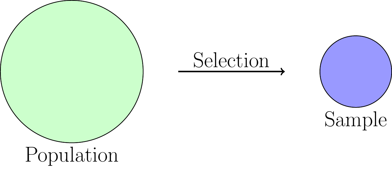
Figure 2.5: Very schematic view of population and sample
Example 2.7 (Poor sampling) We consider two examples. Think through why the sampling procedure is not likely to give a representative sample in each case.
You want to estimate on average how much time a person in Molde spends on shopping per week. You decide to select your sample by going to a shopping centre (where you are sure to find people) at mid-day. You ask a few questions to 100 persons and start to analyze your data. Will you get a representative sample of the population of people in Molde?
You want to survey a (human) population’s average spending on mobile phone services. You invite people through ads where they can either scan a QR-code or use a web address to connect to a web-based survey that you carefully made. Will you attract a representative sample of all mobile phone users?
(A QR code looks something like the picture below and usually represents a link to some web adress. The code can be scanned with a smartphone and connection can be made immediately.)

We will for the most part of these chapters assume that our samples are sufficiently representative of the populations we study.
Most of the information we seek will be in terms of parameters of a population. For instance, in example 2.7 above, about shopping, we would likely denote by \(\mu\) the mean time spent shopping per week for the whole population. Based on a sample we get \(n\) different individual values, from which we calculate the sample mean \(\bar{x}\). If the sample is representative, \(\bar{x}\) is our best guess for the value of \(\mu\). We call the number \(\bar{x}\) an estimate. Since the estimate is based only on a sample it is clear that in general, \[ \bar{x} \ne \mu\;, \] i.e. the estimate is basically never equal to the true parameter value. On the other hand, we feel that for large samples the estimate should be close to the parameter value. But how close? That is precisely what statistics can tell us. We will see some answers to that shortly. It is perhaps remarkable that we can answer such questions at all, since we after all have only one sample value \(\bar{x}\).
The key idea that makes statistics work is the following. Without looking at the value of an estimate like \(\bar{x}\) we can consider the process of (i) taking a sample from a population, and (ii) computing the sample mean — as a random experiment. In this view, \(\bar{x}\) can be considered as a random variable. In this context we call \(\bar{x}\) a statistic. The probability distribution of the statistic is what we use when we deduce how close an estimate is from the parameter we seek to estimate. It is called the sampling distribution of the statistic. Even though it can be considered fundamental to a complete understanding of statistics as a subject, we will not go in detail about analyzing sampling distributions. The results we use in this text are however deduced from certain sampling distributions as we will see.
2.8.1 Confidence intervals
As seen above, we estimate a population mean \(\mu\) with the sample mean \(\bar{x}\). The precision of the estimate is expressed by a confidence interval. For this, we need to set a confidence level, say we want 95% as confidence level. Given this level, we want to determine a margin of error , labeled \(\mbox{ME}_{95}\). This means that we want \[ \bar{x} - \mbox{ME}_{95} \leq \mu \leq \bar{x} + \mbox{ME}_{95} \] with probability 0.95. This would constitute what we call a 95% confidence interval for \(\mu\). Given a sample of size \(n \geq 30\), one finds the following expression for the \(\mbox{ME}_{95}\). \[ \mbox{ME}_{95} = z_{_{0.025}} \frac{S}{\sqrt{n}} = 1.96 \frac{S}{\sqrt{n}} \] The \(z_{_{0.025}}\) value is the particular cut-off value for \(N(0,1)\) that cuts off 2.5% to the right. In other words, the 95% remains between \(\pm z_{_{0.025}}\). The \(S\) value is simply the sample standard deviation, and \(n\) is the sample size.
We follow up with the common generalization, where a so-called significance level \(\alpha\) is used. This is a relatively small probability, given in advance. It is almost always one of the values 0.10, 0.05, or 0.01, and in most cases it is 0.05. The connection between \(\alpha\) and the confidence level is simply as follows. \[ \mbox{ Confidence level $= 100( 1- \alpha)$} \;. \] The general formula then, for a \(100(1 - \alpha)\%\) confidence interval for a mean \(\mu\) is \[ \bar{x} \pm z_{_{\alpha/2}}\frac{S}{\sqrt{n}} \;. \] This is valid for samples of size 30 or more. We will come back to the case where \(n < 30\) in later chapters.
| Confidence level | Significance level \(\alpha\) | \(z_{_{\alpha/2}}\) |
|---|---|---|
| 90 | 0.1 | 1.64 |
| 95 | 0.05 | 1.96 |
| 99 | 0.01 | 2.58 |
Table 2.1 gives the connection between \(\alpha\) and confidence levels, and also shows the corresponding values for \(z_{_{\alpha/2}}\).
Example 2.8 (Confidence interval for a mean) At a salmon farm there can be several thousand fish in each feeding compartment. When the fish in a particular compartment reaches a certain mean weight, they are ready for being processed to food. Suppose the limit is 2.5 kg. It means that the manager who decides when to take out the fish needs to be fairly certain that the (unknown) mean \(\mu\) of the fish is greater than 2.5;. To find out about this, a sample of \(n = 50\) fish is taken. The mean weight in the sample was \(\bar{x} = 2.61\)kg and the standard deviation was 0.25kg. The manager wants a 95% confidence interval for \(\mu\) to assist in the decision. With the given numbers, we take \(\alpha=0.05\), and we find \(z_{_{\alpha/2}}= z_{_{0.025}} = 1.96\). The limits in the confidence interval is thus \[ \bar{x} \pm z_{_{0.025}} \cdot \frac{S}{\sqrt{n}} = 2.61 \pm (1.96) \cdot \frac{0.25}{\sqrt{50}} = \begin{cases} 2.54 \\ 2.68\;. \end{cases} \] With confidence level 95% we can make the claim that \(\mu\) is between 2.54 and 2.68. In particular there is fairly strong evidence from the sample that \(\mu > 2.5\), so based on this, the manager will decide to start processing the fish.
The example shows how even very basic statistics can be used for business decision support. It greatly reduces the uncertainty about the amount of fish that can be produced from this particular compartment. There are two trade-offs that must be handled by the decision maker in such cases.
- Confidence level: Setting this level is part of a “policy” for risk management in the business. Clearly, it feels better to be 99% sure about something than 95% sure. However, increasing the confidence level comes at the cost of increased error margins — i.e. lower precision in statements. Just see how the \(z_{_{\alpha/2}}\) factors increase in table 2.1.
- Sample size: Choosing the sample sizes used for gathering data is part of the same policy. Clearly, larger samples give better information and less uncertainty. However, sampling is a cost and must be limited.
From the formula for error margins, we see that to double precision, we need to four-double sample size. This is because of the square root of \(n\).
The basic “cycle” of statistical analysis and inference is illustrated in figure 2.6. Through sampling and analysis we are able to make statements regarding unknown parameter values in a large population.
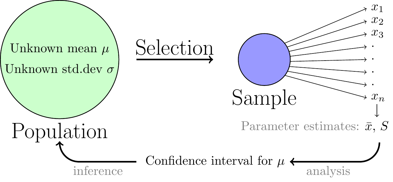
Figure 2.6: View of the inference process for a simple confidence interval.
2.8.2 Proportion confidence interval
We now proceed to the question of how to estimate a population proportion. Let us make sure we agree what this means. We consider a population where the objects belong to one of two groups, \(A\) or \(B\). Let \(N\) be the total population size, and let \(N_A, N_B\) be the sizes of the two groups. Suppose we are interested in the proportion \(p\) of the whole population that belongs to \(A\). Obviously, \[ p = \frac{N_A}{N}\;, \] but the typical problem is that we do not know \(N_A\) or even \(N\). To determine \(p\) exactly would take a complete examination of the whole population, which is often not practically feasible. This means we need to take a small sample of the population and estimate \(p\) from the sample. It is fairly obvious how to compute the point estimate, which will be called \(\hat{p}\). But how do we find error margins for this estimate? We will see shortly, but first a few examples where such estimation is relevant.
Example 2.9 (Estimating a proportion)
- The salmon farm previously visited has problems with some genetic defect present in a proportion \(p\) of the 2012 generation of salmon. The condition makes these fish unusable as human food. The management needs good estimates of \(p\). The detection of the defect requires a thorough dissection of each fish, so completely surveying the whole population is out of question. A sample must be examined, and \(p\) must be estimated from this. Here the group \(A\) are the fish with the defect.
- To monitor the political landscape in a country, one regularly conducts sampling to find estimates of the proportion of voters in favor of different political parties. Such information is in demand from mass media, and from various political groups. Here, the population is all voters, and the group \(A\) are those in favor of the party in question.
Now let’s have a look at some details about the estimation of proportions. We consider a population, where a proportion \(p\) belongs to the \(A\) group. We have a representative sample of size \(n\) from this population. Let \(n_A\) be the number of sampled objects belonging to group \(A\). Then the only reasonable estimate for \(p\) is \[ \hat{p} = \frac{n_A}{n}\;, \] i.e the sample proportion. We need to make an assumption that the sample size \(n\) is not too small. Formally, assuming \(n\) is large enough to ensure \(n\hat{p}(1-\hat{p}) > 5\) we can work with the following error margins in a \((1 - \alpha)100\%\) confidence interval for \(p\). \[ \mbox{ME}_{\hat{p}, (1-\alpha)100} = z_{_{\alpha/2}}\sqrt{\frac{\hat{p}(1-\hat{p})}{n}}\;. \] Here we use the general notation \[ \mbox{ME}_{\hat{p}, C} \] to denote the error margin for the estimate \(\hat{p}\) at confidence level \(C\). In the same notation we could write for example \[ \mbox{ME}_{\bar{x}, 95} = 1.96 \frac{S}{\sqrt{n}}\;. \]
Let us do an example.
Example 2.10 (Confidence interval of proportion) Consider the proportion \(p\) of salmon with the genetical defect, from example 2.9. The management wants to estimate \(p\) and to have a 95% confidence interval. If the lower limit of the interval is above 0.10 (10%) they will consider not to produce the fish to human food. Suppose in a sample of \(n = 230\) fishes there were 30 with the defect. We will find a 95% confidence interval for \(p\) based on that sample. First we find \[ \hat{p} = \frac{n_A}{n} = \frac{30}{230} = 0.130\;. \] Then check that \(n\hat{p}(1-\hat{p}) \approx 26 > 5\) so that we can use the above formula. Then it is a simple computational matter to arrive at limits \[ \hat{p} \pm \mbox{ME}_{\hat{p}, 95} = \hat{p} \pm z_{_{0.025}} \sqrt{\frac{\hat{p}(1-\hat{p})}{n}} = 0.130 \pm 0.043 = \begin{cases} 0.087 \\ 0.174\;. \end{cases} \] Even though the estimate is above 0.10, the lower limit is 0.087 so there is a fair chance that the true \(p\) is below 0.10, i.e. no strong evidence that more than 10% of the population is affected by the problem. ****
We conclude this section with the inclusion of a standard normal probability table.
To be completely correct, there is another subtle condition that needs to be satisfied, namely that \((X,Y)\) has a multidimensional normal distribution. This will always be the case in our work, given that \(X\) and \(Y\) have normal distributions.↩︎