Chapter 8 Logarithmic transformations
8.1 Introduction
The traditional linear model \[ Y = \beta_0 + \beta_1 X + \mathcal{E} \] supposes a unit change in the independent variable leads to a fixed average change of size \(\beta_1\) in the dependent variable. This is not a always realistic model. Two simple examples can immediately be brought up;
A. In classical economic theory, it is generally assumed that a 1% increase in the price of a commodity leads to a certain fixed percentage \(a\) change in the demand for the commodity, if all other factors are fixed. If \(Y\) is the demand, and \(X\) is the price, this leads to a model of the form \[\begin{equation} Y = c X^a\;. \tag{8.1} \end{equation}\] Here \(c\) is another constant, relating to the size of the market. In economics, \(a\) is known as the elasticity of demand with respect to price, or just the price elasticity. The model (8.1) is often called the constant elasticity model.
- In a market for used cars (and many other used products), it natural to assume prices to drop with a fixed percentage per year of age (rather than a fixed amount). So if \(Y\) is the selling price, \(X_N\) is the price of the car when new, and \(X_A\) is the age, we could describe the relation as \[\begin{equation} Y = X_{_{N}}r^{X_A}\;, \tag{8.2} \end{equation}\] where \[ r = \left( 1 - \frac{p}{100} \right) \] is the price reduction factor. In this notation, \(p\) is the annual percentage price loss. This is a more realistic model than the linear model we previously studied for car prices.
In example A, a percentage change in \(X\) leads to a fixed percentage change in \(Y\). In example B, a unit change in \(X_A\) leads to a fixed percentage change in \(Y\). In both examples, we end with a non-linear model for the dependency. If in example A, the elasticity \(a\) is known, we can use the trick from chapter 7, and introduce a new variable \[ Z = X^a \;, \] and then note that \(Y\) depends linearly on \(Z\). Likewise, in example B, if the percentage \(p\) - and thus the factor \(r\) - was known, we could resolve the nonlinearity in a simple way. In practice, though, such parameters are almost never known exactly. Instead, we have to resort to some estimates. Then the question is exactly: Given data for the involved variables, how can we come up with estimates?
The answer - and the solution - lies in a different way of linearizing this type of models. It uses what is called logarithmic functions. These are just a special type of mathematical functions with certain nice properties that can help us out of the problems in examples A and B. Before going into the more technical detail around logarithmic functions, let us consider a specific data example that illustrates what we are after in this section.
:::{.example label = “expodata”, name = “The effect of logarithmic transformation”}
Suppose we observe the demand for some commodity along with the price for a number of periods, and plot the corresponding points to obtain a scatterplot as shown below. Demand and price should follow the law outlined in example A above, but of course other factors can come into play, so we observe some randomness in the data, as shown in the left part of figure 8.1. What we would want to do is to estimate the demand curve, and in particular the price elasticity, based on such data. Now, this curve would look something like what we see in the right part there, and certainly we can not directly apply linear regression to this case.
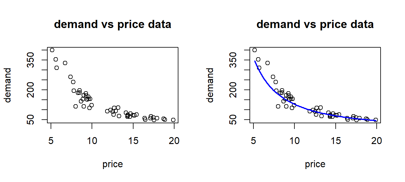
Figure 8.1: Raw price and demand data.
:::
What we are going to do in this chapter, is to outline how logarithmic transformation of both price and demand makes the relationship linear, and so we can estimate parameters with linear regression. For now, we can simply calculate log(price) and log(demand) and make a plot of the resulting variables. We get the picture on the left side of figure 8.2. What we see is a typical linear relation between these new variables, and we can estimate the regression line as in the left picture. Part of the “magic” we will see, is that the slope of this line (which we easily estimate) is exactly the price elasticity.
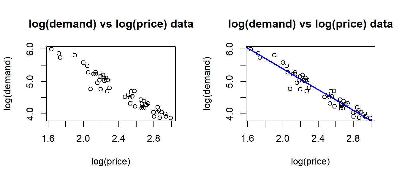
Figure 8.2: Transformed data.
8.1.1 Logarithmic functions
All logarithmic functions are defined for positive numbers \(x\), and they share two fundamental
properties: If \(a \geq0\) and \(b\) are any numbers, and \(f\) is a logarithmic function, we will have
\[\begin{eqnarray}
% \nonumber to remove numbering (before each equation)
f(a\cdot b) &=& f(a) + f(b)\;, \tag{8.3} \\
f(a^b) &=& b\cdot f(a)\;. \tag{8.4}
\end{eqnarray}\]
The trick regarding our models is to transform the relation by applying such an \(f\) function to
both sides of the equation. As we will see, the two properties above will lead to a completely
linear relation between the logarithms of the variables. To keep things as simple as possible,
we will stick to one single logarithmic function, called the natural logarithm function. Usually
this function is referred to as \(f(x) = \ln (x)\). It is sometimes called the “base-\(e\)” logarithm.
We use this function to transform parts of a model into linear terms. Any statistical software
has a built-in version of the function that we can use in practical calculations, to transform variables in a data set.
The function in R is called log, in Excel it is called “LN”.
8.1.2 Resolving non-linearity with \(\ln\) for example A
Suppose now that \(f(x) = \ln(x)\). This function has the two properties shown in (8.3) and (8.4) above.
Starting with example A, let us see what happens when we apply the function to both sides of equation (8.1). The first fundamental thing to recall, is if we apply the same function to both sides of an equation - it remains an equation. Then by using (8.3) and then (8.4), it follows that \[\begin{align*} f(Y) & = f(c X^a) \\ & = f(c) + f(X^a) \quad \\ & = f(c) + a \cdot f(X) \;. \\ \end{align*}\] Now, rename constants and variables as follows. \[ U = f(Y), \quad b= f(c), \quad Z = f(X)\;. \] Then by the calculations, we can write the transformed equation as \[\begin{equation} U = b + aZ \;. \tag{8.5} \end{equation}\] This is obviously a linear relation between new variables \(U\) and \(Z\). Since all \(Y\) and \(X\)-data can be transformed with the \(f(x) = \ln(x)\) function in your , we can directly estimate the coefficients \(B\) and \(a\) in the transformed model. Usually, we will just write the transformed model as \[ \ln(Y) = \ln(c) + a \ln(X)\;. \] We note that the elasticity \(a\) from the original model appears in original form, while the constant \(c\) is transformed.
8.1.2.1 Reverse transformation
Suppose we transformed the original demand model to arrive at equation (8.5). We could then
estimate the coefficients \(b\) and \(a\) in that model. How do we get back to the original parameter \(c\)? To answer this, we
have to resort to the definition of the \(\ln\) function. This is in fact the inverse function to the base-\(e\) exponential
function. With \(e\) equal to the natural constant \(e = 2.71828...\) we have in general
\[ b = \ln (c) \ \mbox{if and only if} \ c = e^b \;. \]
So, this simply means, if we have a value - or an estimate - for \(b\), and \(b = \ln(c)\), we can find the corresponding value for
\(c\) as
\[ c = e^b\;. \]
All calculators has the \(e^x\) function built in, sometimes labeled as EXP(x) or \(\exp(x)\). Moreover, all statistical software has this function,
in R it is exp, in Excel we can use “EXP”.
Supposing we find an estimate \(\hat{b} = 0.34\) for \(b\), the corresponding estimate for \(c\) is then \[\hat{c} = \exp (0.34) = e^{0.34} = 1.405\;. \]
8.1.3 Resolving non-linearity for example B
For model @ref{eq:price-drop-percent), we will benefit from an initial change of variables. Divide both sides by \(X_N\) to arrive at \[ \frac{Y}{X_N} = r^{X_A} \;, \] so instead of looking at price \(Y\) as the dependent variable, we look at price relative to new-price as dependent. Let \[ V = \frac{Y}{X_N} \] denote the new dependent variable, so that the model now reads \[ V = r^{X_A} \;. \] Now, using \(f(x) = \ln(x)\) on both sides of the equation, we get to \[\begin{align*} f(V) & = f( r^{X_A}) \\ & = X_A\cdot f(r) \\ & = f(r) \cdot X_A \;. \end{align*}\] Now, rename constants and variables as follows. \[ U = f(V), \quad q= f(r), \quad Z_A = X_A \;. \] Then the equivalent linear model is \[\begin{equation} \tag{8.6} U = q Z_A \;. \end{equation}\]
Which is a linear model with 0 constant term. There are ways to estimate models with this property. Note the difference from example A: Here the \(X_A\) variable is not transformed, only the dependent variable appears in logarithmic form.
8.1.4 Modeling randomness in exponential models
So far, we have not included random errors in the examples. These are commonly assumed to appear as multiplied factors rather than additive terms. I.e. in example A one would typically model error as \[ Y = c \cdot X^a \cdot \mathcal{E} \;, \] where \(\mathcal{E}\) is a random factor, now typically with mean value 1. The logarithmic transformation now reads \[ \ln(Y) = \ln(c) +a \ln(X) + \ln(\mathcal{E}) \;, \] or, defining \(\mathcal{U} = \ln(\mathcal{E})\), and using \(U, Z\) and \(b\) as above, we get \[ U = b + a Z + \mathcal{U} \;. \] The awake reader now recognizes this as exactly a classical linear regression model. It is in this form of the model we really consider the estimation of the coefficients \(b, a\) and this is can be done precisely as before with R, on the transformed variables corresponding to \(U\) and \(Z\). Anything we learned about basic linear regression can now be applied to the estimation of this model, for example we can find confidence intervals and do tests for the real \(a\) parameter. Recall that \(a\) is still the price elasticity from the original model. So, now we know - at least in principle - how to estimate price elasticities.
A similar approach is used in example B, leading to the extension \[ U = q Z_A + \mathcal{U} \;. \] of model (8.6).
8.1.5 Extending to multiple models
The models examined so far has involved only one independent variable. Of course, models like the one in example A can involve several independent variables. Suppose a company is selling some product or service, and the price is a variable \(X_1\). Suppose \(Y\) is the demand. If there are, say, 2 other competing products with prices \(X_2, X_3\) a reasonable model would be \[\begin{equation} Y = c X_1^{a_1} X_2^{a_2} X_3^{a_3} \cdot \mathcal{E}\;. \tag{8.7} \end{equation}\] Applying the \(\ln\) function to both sides, will after repeated application of the two properties (8.3),((8.4) give the following form: \[ \ln(Y) = \ln(c) + a_1 \ln(X_1) + a_2 \ln(X_2) + a_3 \ln(X_3) + \ln(\mathcal{E}) \;, \] which we recognize as a linear multiple regression model for the transformed variables.
Suppose the market for the product is seasonal, and you want to allow to estimate a possible difference between, say, summer and non-summer market conditions. let \(S\) be a dummy variable indicating observations in the summer, i.e. \(S = 1\) for summer data, \(S = 0\) otherwise. Then consider the model \[\begin{equation} Y = c r^{S} X_1^{a_1} X_2^{a_2} X_3^{a_3} \cdot \mathcal{E}\;, \tag{8.8} \end{equation}\] where now \(r\) is another parameter. Note for this model, that the factor \[ r^S \] is either equal to 1, when \(S=0\), or equal to \(r\) when \(S = 1\). So if \(r = 1. 15\), the model describes a general increase in demand by \(15\%\) in summer, compared to other seasons. Now, the point is that \(r\) will not be known, but appearing in the model as a parameter, it may be estimated. For that purpose, note how the term is transformed into \[ \ln(r) \cdot S \] by the logarithmic transformation, so it fits with the linear structure of the transformed model. The whole model (8.8), after transformation is \[ \ln(Y) = \ln(c) + \ln(r) S + a_1 \ln(X_1) + a_2 \ln(X_2) + a_3 \ln(X_3) + \ln(\mathcal{E}) \;, \] So, if we find an estimate for \(\ln(r)\) at, say, 0.20, we get an estimate for \(r\) itself through the exponential function, \[ \hat{r} = \exp(0.20) = e^{0.20} = 1.22 \;, \] i.e. an estimated 22% increased demand when \(S = 1\), i.e. summer season in this example.
Without specifying further detail, we realize that many different time-dependent demand variations can be specified and estimated, using dummy variables as above. For instance, demand for bus tickets Molde - Trondheim would almost certainly be higher on Fridays and Sundays. The presence and magnitude of single day demand peaks can easily be estimated along with price elasticities, using modeling tools as shown above.
8.1.6 Why estimate price elasticity
So far, we have seen how to estimate price elasticities. We have not raised the fundamental question why estimate price elasticities. For students with an academic background from economics, the motivation should be fairly obvious. Let us just point to the basic motivation. Just look at a single-price model, \[ y = c x^a\;. \] where now \(y\) is demand, \(x\) is the price. It represents the expected demand as a function of price, i.e \(y\) is (expected) number of units we sell at price \(x\). In normal markets, the elasticity \(a\) is a negative number, meaning higher price leads to lower demand. Since direct revenue \(R\) from sale is given by \[ R = y \cdot x = cx^{a + 1}\;, \] we see that revenues can be increased by increasing price exactly when \[a+1 > 0,\ \mbox{i.e. when} \ -1 < a \;. \] This is also intuitively clear, since \(a\) represents the percentage reduction in demand when prices increase by 1%. So if for example \(a = -0.6\), we can sell 0.6% fewer units, at 1% higher price, which means revenue increases. Revenue in itself is not that interesting to a business. What matters in the end is profit, i.e. revenue minus cost. Clearly, meeting increased demand comes at a cost. If the cost of supplying an additional unit is larger than the revenue from selling this unit, we should not supply that unit. In other words, our price \(x\) should not lead to higher marginal cost than our marginal revenue at price \(x\). Under normal circumstances, the optimal (profit maximizing) price is when marginal revenue equals marginal cost. Clearly marginal revenue depends directly on the value of \(a\), and hence to determine a near-optimal price, we need to have at least a good estimate for \(a\). As a simple concrete example, suppose we have constant marginal cost \(K\) for supplying the product, meaning that new units can be supplied at cost \(K\) per unit. Let \(R(x)\) denote revenue, and \(C(x)\) denote cost, as functions of price \(x\). One can then find that if \(a < -1\), the theoretical optimal price is \[\begin{equation} x^* = \frac{Ka}{a+1}\;. \tag{8.9} \end{equation}\] So, if \(a = -2.0\), the optimal price would be \(2K\), twice the unit cost of supply. A few remarks can be made about such calculations.
- We use models here, at two or more levels: The relation between demand and price is one model. Secondly, a model for the cost is used to come up with the optimal price. We remember that all models are “false” as they simplify often complex realities. Clearly, the relevance of our calculations always depends on model correctness.
- The demand model may be a good fit in an interval of prices. If the calculated price \(x^*\) is outside this interval, the reliability of the model, and consequently all calculations based on it, is highly questionable.
- Note that if \(-1 < a < 0\), then \(x^*\) in the formula becomes negative, i.e. a meaningless price. In fact, in this situation - and if we believe the demand and cost models to be true for any price - we can always increase profit by increasing prices. That means there is no optimal price. Clearly these models are too simple in this case.
The remarks reminds us about the need for caution in applying models to assist our decisions, for instance pricing decisions in supply chain management. Used with some care however, regression models are great tools to assist decision makers, by providing estimates of central market parameters like price elasticities - as exemplified above.
8.2 Practical considerations - using R
Suppose we are in a situation where we have price and demand data in a data set. The method outlined above suggest we compute new variables for the transformed data, and then apply linear regression to those variables. This is indeed a way that will work in any statistical software system (including R of course.) The case is however, that R offers an even simpler way of getting the estimated transformed model. We now outline the procedure with an example.
Example 8.1 (Demand vs. price of meat.) A supermarket sells two brands of ground meat, A and B. Brand A is cheaper, and brand B is considered a quality brand. Imagine the supermarket have fixed prices for each week, then possibly change it between weeks. Weekly sale volumes in kg, of each brand are recorded along with prices for each brand. Let \(y_A, y_B\) be the sale volumes for brand A, B, while \(x_A, x_B\) are prices in the same week. The classical (one-dimensional) demand model for brand A, says \[ y_A = c_A x_A^{\alpha_A}, \] where \(\alpha_A\) is the price elasticity. Logarithmic tranformation as above gives \[\begin{equation} \ln(y_A) = \ln(C_A) + \alpha_A \ln(x_A)\;. \tag{8.10} \end{equation}\]
We will estimate \(\alpha_A\) and the corresponding \(\alpha_B\) below. First, let’s take a look at the data.
##   saleA saleB priceA priceB
## 1   845   115    110    139
## 2   833   121    124    139
## 3   845   162    116    149
## 4   951   119    105    149
## 5   878   117    108    119
## 6 1006 170 108 119## [1] 50with(meatdata, plot(priceA, saleA, main="brand A"))
with(meatdata, plot(priceB, saleB, main="brand B"))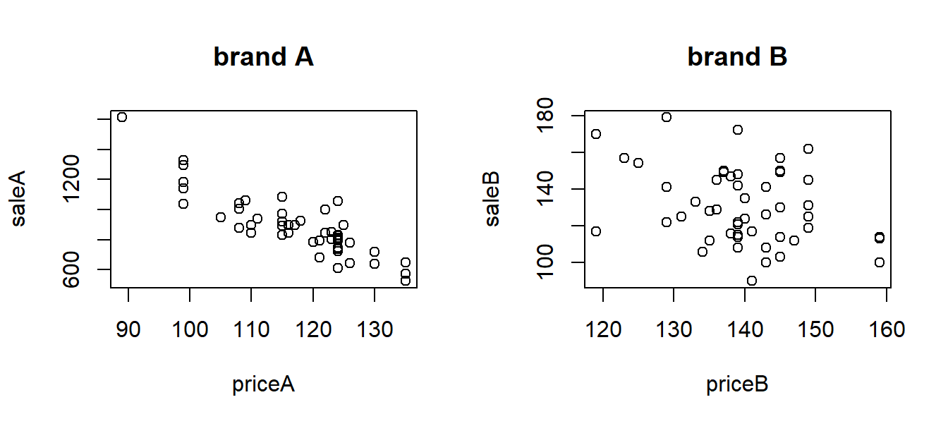
From the plots, it seems that sales for brand A is more affected by the price than brand B.
So, now - let’s run the regressions. Here, we can ask R to simply insert the \(\ln(y), \ln(x)\) from equation (8.10) directly in the regression. In R the natural logarithm is called log, so it looks as follows where we do both brand A and B estimations.
library(stargazer)
#run regressions on log(variables):
logregA <- lm(log(saleA) ~ log(priceA), data = meatdata)
logregB <- lm(log(saleB) ~ log(priceB), data = meatdata)

#show results
stargazer(logregA, logregB, type = "text", keep.stat = c("rsq"))
##
## ========================================
## Dependent variable:
## ----------------------------
## log(saleA) log(saleB)
## (1) (2)
## ----------------------------------------
## log(priceA) -2.018***
## (0.171)
##
## log(priceB) -0.823**
## (0.334)
##
## Constant 16.372*** 8.921***
## (0.815) (1.652)
##
## ----------------------------------------
## R2 0.744 0.112
## ========================================
## Note: *p<0.1; **p<0.05; ***p<0.01We see from the results that the prices significantly affect sales for both brands, with a much stronger effect for brand A (look at the \(R^2\).) The estimated price elasticities are \[ \alpha_A = -2.02 \ \ \alpha_B = -0.82 \] This means a 10% percent rise in prices is expected to cause about 20% drop in sales for brand A, while a 10% rise in the price for brand B is expected to cause about 8% drop in sales. We can look at the confidence intervals (95%). As we also see from the standard errors in regression, the uncertainty is larger in the B brand estimates.
##                 2.5 %    97.5 %
## (Intercept) 14.733526 18.010147
## log(priceA) -2.361989 -1.674147## 2.5 % 97.5 %
## (Intercept) 5.600388 12.2418379
## log(priceB) -1.495541 -0.1506365We can try to plot the estimated demand curves. For brand A, that means we must get back from \(\ln(y_A)\) to \(y_A\). We then use the fact that we have estimated
\[ \ln(C) = 16.37, \alpha_A = -2.02\;, \]
so we get
\[ y_A = \exp(16.37) x_A ^{-2.02} \]
and a similar expression for \(y_B\). Using R we can do something like below. We first plot the observed points, then add the estimated demand curves.
#allow side-by-side plots
par(mfrow=c(1,2))
#get min and max price
m <- min(meatdata$priceA)
M <- max(meatdata$priceA)

#do the plotting
with(meatdata, plot(priceA, saleA, main="brand A"))
curve(exp(16.37)*(x)^-2.02,
      add = TRUE,
      from = m,
      to = M,
      lwd = 2,
      col = "blue")

#repeat for brand B
m <- min(meatdata$priceB)
M <- max(meatdata$priceB)
with(meatdata, plot(priceB, saleB, main="brand B"))
curve(exp(8.92)*(x)^-0.823,
      add = TRUE,
      from = m,
      to = M,
      lwd = 2,
      col = "blue")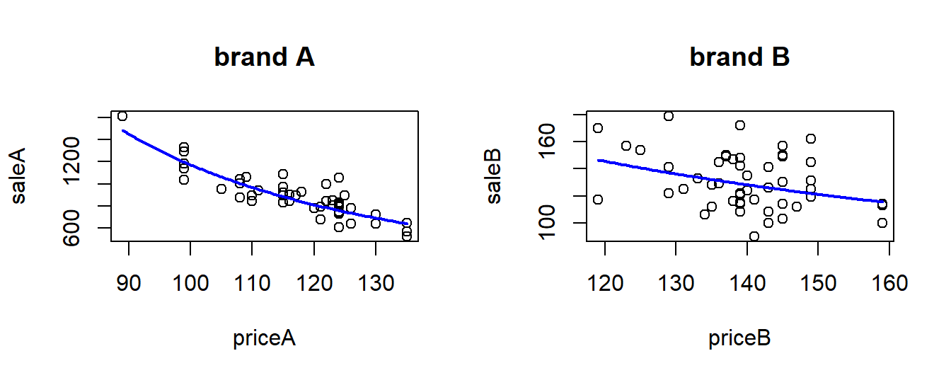
As an intelligent reader, you will notice that the two brands are actually to some extent substitutes for each other, and so the demand for say brand A should in fact depend on both prices (ehh..why?), i.e. we should have as a more satisfying model \[ y_A = C_A x_A^{\alpha_A} x_B^{\alpha_B}\;, \] and a corresponding model for brand B sales. If time permits, we will do an exercise in the course to try to estimate parameters for this model, for both brands.