Chapter 7 Non-linear regression models.
Exercise 7.1 In this exercise, you should try to work along the lines of example outlined in the section on dummy variables in chapter 7. In the second part, you will go even further with the data material. The data are in flat_prices.csv.
- Find and read your copy of the data file. For each of the three towns, compute dummy variables. Use the names
- DMOL for Molde
- DKSU for Kristiansund
- DASU for Ålesund
(So that DMOL = 1 for all flats in Molde, 0 otherwise etc.)
- Run the model that explains most price variation - without taking town differences into account. Include only significant \(x\) variables.
- As a variation to the example in the text, try to include town dependency, but use Kristiansund as the reference category (reference market). Find the estimated model that include all - and only - significant \(x\) variables. Call this model “PRK” (Prices with Reference Kristiansund).
- Call the model from the text (where Molde was the reference category “PRM.” Is there any differences in explanatory power/prediction quality between PRK and PRM?
- Compare the coefficient estimates for the variables that are common to PRM and PRK. Are there large differences? Why are the constants so different? Find the connection between the two constant estimates and the estimated coefficient for DMOL in model PRK.
- Consider an example flat A with the following characteristics
- area = 90 sqm, #rooms = 3, standard = 3
- town = 1 (Molde), distance to center = 3 km
- location = 8, age = 25, rent = 2500 NOK.
Produce price forecasts for this flat using PRK and then using PRM. The price forecasts should be similar. Are they?
- What are the estimated average difference in prices between Molde and Kristiansund? Between Ålesund and Kristiansund? And between Molde and Ålesund? Which are significant?
- (Theory question, use paper and pen.) Suppose \(Y\) = price and \(X_1\) = area in the model PRK, and \(X_i\) denotes other significant original variables. Then the model reads \[ Y = \beta_0 + \beta_1 X_1 + \beta_2 X_2 + \cdots + \beta_{M} DMOL + \beta_{A} DASU + \mathcal{E}. \] Here town dependency is modeled only as a direct level shift. The marginal square meter price \(\beta_1\) is assumed the same for all towns. Still using Kristiansund as reference market, write down a model allowing different square meter prices in different towns. (Hint: See the section on interaction effects.)
- If you found a satisfactory answer to the above question, try to use R to estimate parameters for the model. Is there any evidence of different marginal square meter prices between towns?
- The variable describing the number of rooms is an ordinal variable with relatively few values. Including this variable in a linear fashion shows no significant effect (when area is also included). Think about ways to include the number of rooms information in the model, using dummy variables. One could use rooms = 1 as reference category. Then use dummy variables e.g. as follows
- R2 indicating rooms = 2,
- R3 indicating rooms = 3,
- R4 indicating rooms = 4,
- R5 indicating rooms \(\geq 5\).
On paper sketch how you could implement general price corrections depending on number of rooms. Also think about how you could model - and investigate - possible different square meter prices depending on number of rooms. If you have time, try to do some experiments in this direction with R, using the available data.
- As a purely theoretical exercise, think about how we could now for instance model a separate marginal square meter price for 3-rooms flats in Molde. This shows that using dummy variables in modeling interaction effects gives possibilities for estimating very specific effects in e.g. an economic market. This level of detail is not relevant in this example, but could be in other examples. Note also that there are only 16 3-rooms flats in Molde in the data set. When the model becomes more detailed, we risk that the estimated effects are backed by very small pieces of the data set. That is also a reason for not having individual dummy variables for rooms = 5, 6, 7 and 8, since there are very few observations here.
Exercise 7.2 We refer to the data in exercise 6.1, Wages.csv. Read this file into a dataframe. The models we previously considered did not include information on gender. The data contains an indicator variable female which is 1 for all female workers, 0 otherwise.
- Along the lines of what we did for flat prices, try to include
femalealong with education and experience in a regression model. What - according to this model - is the difference between male and female wage levels? - Make a scatterplot of wage vs. education, with colors based on gender. Something like below will work using
ggplot, assuming the dataframe iswages.
library(ggplot2)
ggplot(wages, aes(x = education, y = wage, color = as.factor(female))) +
  geom_point(size = 2, alpha = 0.5) +
  geom_smooth(method = lm, se = FALSE)
## `geom_smooth()` using formula 'y ~ x'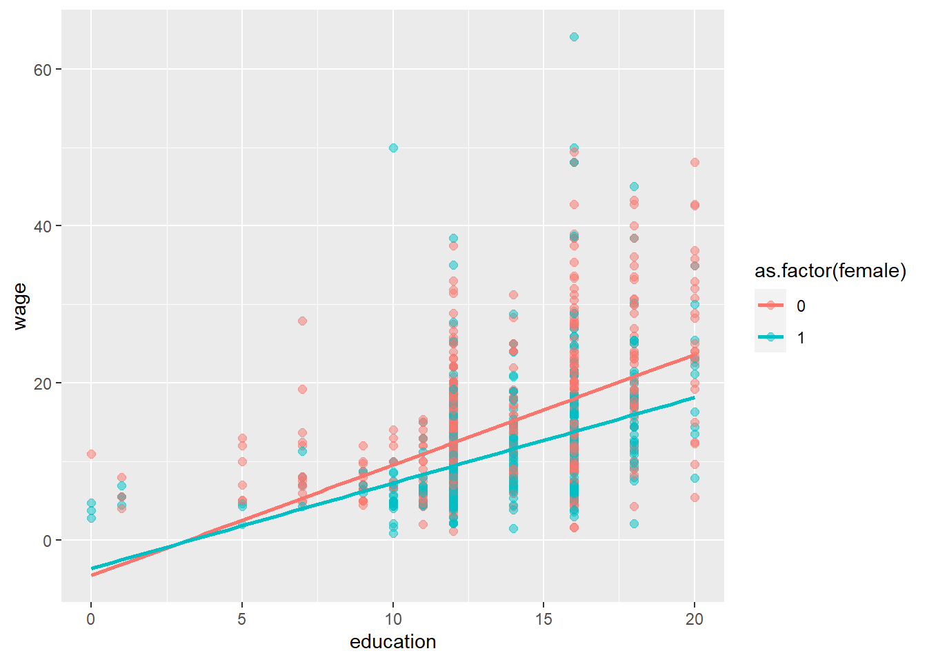
What do we see from the regression lines?
From the plot it appears that males are gaining more from extra years of education than females. This would be an interaction effect. We can estimate interaction effects in some different ways, One way would be to compute a new variable that is the product of female and education and add this in the regression. As is often the case, R provides a direct way: So suppose we want to estimate separate effects of education and gender, plus the interaction of those two, in addition we want the experience in the model. We can use the following code.
wagereg <- lm(wage ~ education*female + exper, data = wages)In the summary, the term education:female represents the interaction effect, i.e. the difference in the education effect between males and females.
Try to run this regression. What is the estimated wage effect of one extra year of education for males? and for females?
Compare forecast wages for Jim and Maria from exercise 6.1 with this model.
The results from these models appear to show a wage discrimination of females, since with the same education and experience we find clear differences in the average wages. Could (parts of) these effects be “false” because of omitted variable bias? Think about some other factors deciding wages that are not included here, and that may be different for males/females. (Remember that the data are from USA 1995).
Include the interaction between
experandfemale. Is this interaction effect significant?