Chapter 3 Introduction to R

Exercise 3.1 The first task is to install and get familiar with R and Rstudio. NOTE: IF YOU ARE WORKING ON A CAMPUS PC - DO NOT TRY TO INSTALL R/Rstudio THERE. Those PC’s already have these programs installed. I.e. the installation part below is only for a PC which does not already run R/Rstudio.

Installation. Go to the canvas room for Log 708 and find the video 1_1_installing_R_project_script.mp4. These video clips are in the module “R introduction videos.” Watch the video either through Canvas streaming or download the video and run it on your PC. You may want to adjust the video settings for optimal screen resolution. (The settings are in the star-shaped icon low right in the video window. You should probably also watch in full screen mode.) Note that the instructions in the video are for a Windows PC. If you run on some other platform (e.g. Mac, linux), there may be some minor differences. Check the web for installation instructions before proceeding to install. If for some reason, you can not make the R/Rstudio installation work despite serious attempts, consider starting with a cloud-based solution here: https://rstudio.cloud/. Here you need to create an account, and then you can run R/Rstudio via a web browser. You get some runtime for free, a small fee buys more time.
First project and Folder structure. Follow the procedure in the video to make your first project. The video creates the first project on the desktop for simplicity. You don’t want to have your files on the desktop in general. You should make sure to have a good structure for all material relating to your master studies, with a folder for Log 708 in a logical place. Try to establish such a structure now, if you did not already do it. If you don’t have a clear picture of how such a structure could look, there is an example folder called MASTER_Coursework.zip in the Other Stuff module in Canvas. You can download and unzip this as a start. Then change and move it as you like. Look to the next point in connection with where you want to have your primary data storage. Note that the MASTER_coursework folder is set up with a few extra folders for other courses in the first semester.
Data safety In relation to the previous task, think about data safety. In this case we mean “how to avoid losing your work/data.” The college offers a safe disk location where you should store any material that you really don’t want to lose. Some of you may have employers that offers a similar backed-up solution. The local disk on your PC can break down and create a “data disaster.” At least with regular frequency make sure you back up your data in a safe place. So, the task here is to figure out in general how you can store data relating to your master studies so that you do not lose them if your PC breaks down, is stolen or simply refuses to cooperate more with you.
Setting default working directory The default working directory is a folder that Rstudio/R will generally use as its working directory. If you start a project, the working directory will be changed to the project folder initially. You can now decide what will be your default working directory. If you used the proposed folder structure from Canvas, there is a ready made folder called myRwork in the LOG708 folder. This could be a good choice as default working directory. Note that you may change this whenever you want. Here is how you do it in the easiest way to begin with. In Rstudio, go to menu “Tools/Global Options…” In the topic “R general” find the field labelled “Default Working Directory (when not in a project).” Choose “Browse..” and find/select the folder that you want to use as default working directory. The result will show the file path to the working directory in the field text. When you are happy, choose “Apply” and “OK.” The file path is a text (in Windows) of type “M:/folderA/folderB/folderC,” it will look similar on MAC. This particular file path means that we have a drive called “M” and on this drive we refer to “folderC” which is in “folderB” which is in “folderA.” More about this later.
Make a project for chapter 3 exercises. It is recommended (though not absolutely necessary) that you collect related work, data and files in an R project as described in the video. So now you can make a project with the aim of collecting all your work on exercises for chapter 3. Make sure you have a dedicated folder for work on these exercises. In the setup from part b. there is already such a folder, with path “…/MASTER_coursework/FirstSemester/LOG708/exercises/chapter3.” Here “…” means something that is specific for your setup. Now in Rstudio, we choose menu “New project….” Choose to create project in existing directory (“directory” means basically the same as “folder”), and browse to where you want it (e.g. the path above if you use that structure). Then choose “create project” and Rstudio will “switch” to work on your new project. Until you close the project, everything you do will be associated with this project. When later you open the project again, all your work will be there ready as you left it. In the file menu you find a few commands relevant to project work. You can “open” a project, “open in new session” if you like to keep your current project active while opening another, and you get a list of recently active projects. When you pause work on a project for some time, it is a good habit to close the project. In the top right corner of Rstudios window, there is also a list of project, so you can quickly switch, open, or close projects. In the project folder, there will now be a file named chapter3.Rproj. This is your project file. You can also activate the project by double-clicking this.

Exercise 3.2 (Getting started with R) In this exercise we start using some of the introductory videos that you find in Canvas. Also, in the Canvas module with the videos, you will find an R.script called LOG708_clips.R. This script contains all of the code that is used in the intro videos. Download from Canvas, and open this script in Rstudio. You can also open a new R script to make your own experiments as you watch the videos. It could be a good idea to save this new script in the “…exercises/chapter3” folder. You could also make this into your current working directory: If you are in a project that is not related to these exercises, choose (in Rstudio) “File/Close Project..” Then choose “Session/Set working directory” and “Choose directory.” Then make your choice. Note that the R code using setwd(...) appears in the console.

Run the video 1_2_Rstudio_interface.mp4. As you watch (or after, if you like) make sure that the codes and tricks used in the videos works in the same way with your Rstudio installation. Note,it is not the point to memorize everything in these videos, its more about getting started, and then as you gain experience and time with Rstudio, you will start getting hold of the most important things.
Make sure you know what the following shortcuts in Rstudio do

    #keyboard shortcut CTRL+ENTER   (Used with the script editor)         
    #keyboard shortcut CTRL+C                
    #keyboard shortcut CTRL+V               
    #keyboard shortcut CTRL+Z (works in the editor only)                
    #Arrow up / down (works differently in editor and console)
    # ALT+"-"

Answers are in the video script file. Start using these shortcuts now!

Watch the video 1_3_operators.mp4 in the same fashion as above, by actively exercising what is shown in the video.
In an R script file, copy in the following comments, and write code that executes what is asked for in the command. So for example if the comment asks

#assign the number 10 to variable named a, and print the value to the console.

you should answer with the following code, which gives the output below in the console.

a <- 10 
a

## [1] 10

Run each answer to check that the code does what it is supposed to do. (recall CTRL + ENTER executes the line where the cursor is in a script file)

Here are some tasks. Copy all the comments here into a new script file, then write code below the corresponding comment.

# assign your year of birth to a variable "year"

# make a vector "date" = (year, month, day) with your date of birth. 
# Recall, there is a super-central R function that creates vectors. 

# make a variable "a" that contains the value (2 + 3)*(10 - 3)^2. 

#assign the value 10 to variable "b" and let z be the sum of a and b. 

#assign the value 1 to "a", 2 to "b", 3 to "c" and 1 to "d".
#you can just overwrite the existing content in the variables. 

#test whether "a" is equal to "b".

#test whether "a"  is not equal to "c".

#test whether "a" PLUS "b" is equal to "c" OR equal to "d".

#assign the numbers 2,3,4 and 5 to "e". (i.e. make a vector)

#assign the numbers 12,13,14 and 15 to "f".

#test whether "a" is element in "e".

#test whether "a" is element in "f".

#make a vector y that contains the product by b of all elements in f. 
#(so, y should be (24, 26, ...), but how to do it most easily with R 
#given that you already defined b and f as variables?)

#show that "f" MINUS 10 is "e". Use the logical comparison "==" in R.

#run ls() in the console to see your workspace variables. See the environment #window (upper right in Rstudio) containing the same, and showing some info.


#run rm(list = ls()) to clear the workspace. Now run ls() again. You can 
#run the whole R script to recreate the workspace variables. (CTRL+SHIFT+ENTER)

#Write ?sum at the console. What happens?

#Create a vector z with 10-15 arbitrary numbers between 0 and 10.

#write hist(z). What happens? In the plots-tab click "zoom". 
#What happens?

#Save your script file with a sensible name in a sensible place,
#congratulate yourself with the excellent work, and take a short
#break:-)

Exercise 3.3 (Some basic functions) We move on to the video 1_4_variables_and_simple_functions.mp4. In the same way as before, watch this video now. You might want to use the same training R script as you created in the previous exercise.

As before, copy the tasks in comments below to a script file, maybe the same as you used before, and write code to execute the tasks.

#make a vector z of 5-10 arbitary numbers. 

#Find the sum of elements in z

#Find the average value of z

#Find the median value of z

#find the mean value of z^2

#make a vector z2 which starts with z but has NA as an 
#additional element. (hint, c(x, y) will put vector y 
# after vector x in a new vector)

#try mean(z2) 

#try mean(z2, na.rm = TRUE)

#In the script editor, write "M <-  med". What happens? Hit TAB. What happens? 

#At the console, write "fact", and use this to find "factorial(10)"
#which is 10*9*8*...3*2*1. Find approximately factorial(100).

Exercise 3.4 (More on R vectors) We continue with the video 1_5_vectors.mp4. After going through the video, do the following tasks in the same way as before.

We start with some more on vector creation.

# clear your workspace. (rm(...) see above if you forgot)

#Use ":" to make a vector x = 4, 5, 6, 7, 8, 9, 10 and a 
#vector y = 100, 99, 98, ...., 3, 2, 1, 0.

# find the length of y. 

# Use "seq" to make a vector z = 1, 4, 7, 10 and a vector 
# w = 10, 8, 6, 4, 2, 0  

# Use "rep" to make a vector x = 1, 2, 3, 1, 2, 3, 1, 2, 3

# Use c(...) to make a vector y that starts with z and ends with w

# Make a vector f1 with 5 uniformly distributed random numbers
# between 0 and 10.

# Make a vector f2 with 5 uniformly distributed random numbers
# between 0 and 10. Is f1 == f2?

# How can we ensure that the randomly generated numbers are 
# the same each time we run our code? And why can this be of
# importance? Make a small sequence of code that ensures 
# reproducible random generation of 5 uniform numbers as above.

Great work! Now, we exercise vector element access methods:

# Define the vector a as follows
a <- c(3, 5, 7, 9, 1, 1)

# extract the third element of a

# extract the vector of all elements of a except the third 

# extract elements in position 2 and 4  

# extract all elements of a that are greater than 3

# try head(a, 3) and tail(a, 3). What do you get?

# change the first element of a to value 1.

# change the second and third element to 0

# Set a back as originally defined. Let b be the vector a backwards
# hint: Google

# What are the vectors a + b, and a*b? Try and see. 

# What is the vector a + 10? Try and see. 

# Find the vectors s1, s2 with elements in a sorted in 
# (1) increasing, (2) decreasing order. 

# What do you get if you try to add x = c(1, 2, 3) 
# and y = c(1, 2, 3, 4)?

Exercise 3.5 (Packages: Install and activate) Before doing this exercise, get familiar with the basics of package installation, shown in (first part of) the video 1_6_packages_saving_loading_data.mp4, and also described briefly in the compendium.

In this exercise we will practice how to install and use R packages. We will also see how we can get hold of data sets stored in R for demo purposes. (This is not the same as reading data from file, which we do in following exercises). We will use a data set called mtcars along with the ggplot2 graphics library.

First, to install ggplot2 run this command:

install.packages("ggplot2")

You usually need to run this command only once on a given PC. That should install the package for later use. You may get some “warnings” from R when doing this, ignore those. If you should happen to get an “error” which you cannot resolve through google or similar, get in touch with someone (teacher, assistant teacher) to try to fix.

Next, in each R session where you want to use the package, you need to activate it. This is done with the library command:

library(ggplot2)

There may be some warning messages, about R versions and such. Ignore those.

So assuming you now have installed ggplot2 successfully, let’s get some data. Here we are going to use a data set called mtcars just for illustration. Since these data are built-in for R, we can use the data function as follows

#include "mtcars" as a dataframe in your workspace
data(mtcars)
#check top 6 rows
head(mtcars)

##                    mpg cyl disp  hp drat    wt  qsec vs am gear carb
## Mazda RX4         21.0   6  160 110 3.90 2.620 16.46  0  1    4    4
## Mazda RX4 Wag     21.0   6  160 110 3.90 2.875 17.02  0  1    4    4
## Datsun 710        22.8   4  108  93 3.85 2.320 18.61  1  1    4    1
## Hornet 4 Drive    21.4   6  258 110 3.08 3.215 19.44  1  0    3    1
## Hornet Sportabout 18.7   8  360 175 3.15 3.440 17.02  0  0    3    2
## Valiant           18.1   6  225 105 2.76 3.460 20.22  1  0    3    1

#get some info about the data
?mtcars

Without going into detail, we see that the data is about cars and fuel consumption, plus diverse characteristics of the cars. Since the point of this exercise mainly is to see how we can install packages, we will not dig deeper into the data, just check that the ggplot function in the package ggplot2 works as intended. Here is an example that you could try to run. The result should look like the figure below the code.

What is roughly the (not unexpected) relationship between weight and horsepower? How is automatic vs manual shift affecting the data? Such visualizations show patterns and relations in data that could otherwise be difficult to spot.

#Redefine variable "am" as a factor, just to make figure labels look right.
shift <- factor(mtcars$am, labels = c("automatic", "manual"))

#make a plot
ggplot(mtcars, aes(x = wt, y = hp, color = shift)) +
  geom_point(size = 3) + 
  labs(title = "Horsepower vs weight", 
       x = "Weight",
       y = "Horsepower")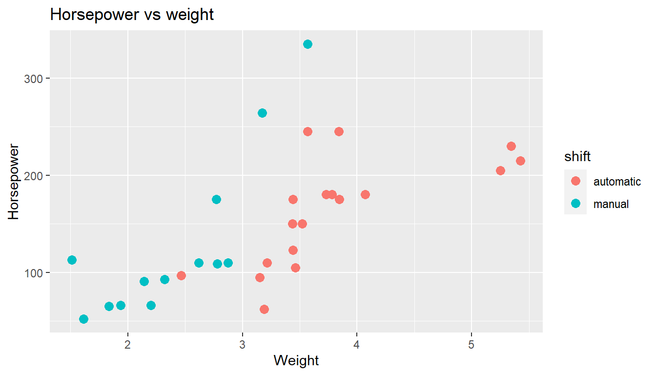

Add the code + geom_smooth(method = lm) to the code above. Can you guess/describe what the new elements in the figure represents? (Don’t worry if you can’t, we will learn later anyway! :-))

Exercise 3.6 (About working directory, reading data files and internal R help.) If not done, watch the remaining part of video 1_6_packages_….

Use the command getwd() to find the path of you working directory. This is a string (a text) looking for example like “M:/MASTER_Coursework/FirstSemester/LOG708/exercises/chapter3” if you have used the proposed folder setup from exercise 3.1 a. and put the main folder on a drive called “M.” It will probably look similar - but not exactly like this on you PC.
If you have not already done so, download the compressed folder log708data.zip (or log708data.7z if you prefer that) from canvas, and extract the files into a logically good place in you LOG 708 folder system. (e.g. into the (empty) log708data folder in the suggested structure). Get help (from a person or the web) if you run into problems.
We now want to read from disk the data file flights_NO.csv. One way we can do this is in Rstudio, go to the menu “File/Import Data….” Since we want a .csv file, choose “From Text (base)….” Now you get to a dialog box, where you can locate the file. Do that. Next, you may adjust some settings to make data look right. Then click “Import,” and you will get the right code into the console. To check that everything is OK, use command ls() to view your workspace, and see that there is a dataframe with the read data there. What is its name? Use head(...) to check the top rows. ( … means the name of the dataframe here). Copy the code with ... <- read.csv("...") into your R script file. You can re-execute the code at any time to read the original data again. Continue writing code in the R script.
Use the code

df2 <- subset(..., Day.of.Week == "Monday" & Seats > 50)

to make a subset of the whole data set. What does df2 contain? How many rows are in df2, and in the original data?

You have now successfully read data into R. Let’s try to write the data in df2 to disk: Try

#write df2 to disk with given file name.
write.csv(df2, "LargeMondayFlights.csv", row.names = FALSE) 

#view the working directory, you should see the new file there:
dir()

See if you can write the data frame df2 to a file with the name “LargeMondayFlights_NO.csv” in your main data folder. (Hint: copy the relevant part of the path that was used when reading the original data.)

You now know something more about reading and writing data from/to disk storage. You can delete the newly created data files if you like, but keep the R code in your R script. (You are working on an R script for this exercise also, aren’t you ?? :-))

Exercise 3.7 (Getting help) In this little exercise we try out some of R/Rstudio’s internal help tools, as well as external (web) sources. One should note that the internal guides in R are often somewhat compact and technical, while on the web you find more detailed examples.

Suppose we want to learn a bit about how R can help us do calculations with normal distributions. Suppose we have a standard normal variable $Z$ and also another normal variable $X$ with mean = 10, and standard deviation = 3.

We want to find out how we can find such things as \[P[Z \leq 2.1], P[Z \geq 2.1], P[X \leq 12], P[8.4 \leq X \leq 10.9].\]

Try to use the internal help system, via ?normal or help(normal) to find the probabilities. You should in this case not use standardization of $X$ for the latter two cases, since there are built in general normal distributions in R.
See if you can find information about the same type of calculations via google (or similar).
Proceed by internal or external help to find a number $b$ such that $P[Z \leq b] = 0.80$.
Can you also find a number $c$ such that $P[X \geq c] = 0.90$?
Can you produce a vector my_x of 30 random numbers from the distribution of $X$? (The same normal distribution). Find the (sample) mean and standard deviation of my_x. Are they close to the real parameters?

Exercise 3.8 (Working with data frames) This exercise is based on topics discussed in the videos 2_1_dataframes_I and 2_2_dataframes_II. We will play with the concept of a data frame in R. We will make our own data. Your workspace is maybe full of things from past exercises. Assuming you saved relevant commands in R scripts, clear the workspace with rm(list = ls()). Check that the workspace is empty.

create a vector a that entails the first names of 10 of your friends, relatives, collegues, etc. MAKE sure to put the code in an Rscript file so you can repeat it.
create a vector b that entails the age of these 10 persons.
create a vector c that entails the hair color of these 10 persons.
create a vector d that entails the number of years you have known these 10 persons.
combine a- d into a dataframe “friends.” (Hint:here and below, you should be able to find a method on the web).
name the columns of “friends” as follows. “name,” “age,” “hair,” “time.”
create data frame “friends2” by subsetting “friends” containing only people younger than 20.
show how many people in “friends” are younger than “20” (i.e. count rows in “friends2”).
create data frame “friends3” by subsetting “friends” containing only people equal or older than 20 AND whom you have known for more than 10 years.
create vector “not_seen” that entails for each of the 10 the number of days you have not seen the individual person.
add “not_seen” as additional column to “friends.”
Take a break. Save all R code if you leave the computer.

Exercise 3.9 (Basic descriptive statistics.) Keep on working on the “friends” data frame. (Rerun the code necessary to generate it if necessary). We’re going to do a little descriptive statistics here.

create a histogram for the variable “not_seen” in “friends” (graphs should have a title and axes should be named).
create a barplot for the variable “hair” in “friends.”
create a scatterplot for the variables “age” on the x-axis and “time” on the y-axis".
save “friends” as a csv-file in your working directory.
import the same data file again as object “friends2.” Check that friends and friends2 are the same data.

Exercise 3.10 (More on descriptive statisics.) Now, before doing this exercise, watch the final intro video, 2_3_finding_NA_plotting_data. We will use data in the file world95.csv which you can find in the main log708 data folder.

read the file into a data frame, called for example w95.
use names(w95) to see what variables there are.
what do you get from ncol(w95) and nrow(w95)?
get a look at the top 10 rows of data.
try View(w95) (note the unusual capital V). What happens? Try to show data in a separate window. (small icon at the top of view window…)
Find mean life length expectancy for males and females. (variables lifeexpm, lifeexpf). (Remember df$x picks out variable x from dataframe df).
find the median values for the two variables above. Does comparing the mean and the median indicate some skewness in the distribution?
make histograms of the two variables, and see if you can explain the difference in mean and median from the figures.
assign to an R variable MM the maximum male lifelength in the data.
find which country (or countries) had the maximum MM (Hint: subset with a condition using == …)
Compare the mean and median population in the sample. What fraction of the countries have less than the mean population. Make a histogram of the population variable that explains the large difference. Hint: use hist(... , breaks = 30) to make the histogram look reasonable.
make a scatterplot of female expected life length vs. literacy. Make sure the plot has a title, and x- and y-axis labels that make sense.
make the same plot as above, but only for countries within OECD. (Hint: With base R, we can simply make a subset of the original dataframe so as to only consider OECD countries. The code will be the same, exept for a different data frame name.)
use table(...) to count the number of observations within each region.
The variable calories shows the daily energy intake per capita. Try to find the mean value of this variable. Why do you get NA? add the option na.rm = T to your mean function call.
The function is.na tests if a value is NA. What do we get if we write table(is.na(w95$calories))? Another way to get the same, perhaps better looking is with(w95, table(is.na(calories)))
Try with(w95, boxplot(calories ~ region)) and zoom the plot. This reveals some striking regional differences. Hopefully the picture is better for current data.