Chapter 3 Introduction to R

Exercise 3.1 The first task is to install and get familiar with R and Rstudio. NOTE: IF YOU ARE WORKING ON A CAMPUS PC - DO NOT TRY TO INSTALL R/Rstudio THERE. Those PC’s already have these programs installed. I.e. the installation part below is only for a PC which does not already run R/Rstudio.

Installation. Go to the canvas room for Log 708 and find the video “R_Studio_installation”. This is found in the Panopto Video section, in the subfolder “Videos on basic R”. Note that the instructions in the video are for a Windows PC. If you run on some other platform (e.g. Mac, linux), there may be some minor differences. Check the web for installation instructions before proceeding to install. After completed installation, start Rstudio and check that it looks as in the video. If questions about update appears, choose “ignore update”.

If for some reason, you can not make the R/Rstudio installation work, consider starting with a cloud-based solution here: https://posit.cloud/. Here you need to create an account, and then you can run R/Rstudio via a web browser. You get a fair amount of runtime for free, a small fee buys more time. The video “Alternative ways to run Rstudio” shows how this works, along with some other options.

Folder structure. Watch the video More about Rstudio. Start Rstudio and have a look along with the video to get familiar with the basic interface. Run a few calculations in the console, try to make an R script, a .R file. You should make sure to have a good structure for all material relating to your master studies, with a folder for Log 708 in a logical place. Try to establish such a structure now, if you did not already do it. If you don’t have a clear picture of how such a structure could look, there is an example folder called MASTER_Coursework.zip (alternatively MASTER_Coursework.7z) in the Other Stuff module in Canvas. You can download and unzip this as a start. Then change and move it as you like. Look to the next point in connection with where you want to have your primary data storage. Note that the MASTER_coursework folder is set up with a few extra folders for other courses in the first semester.
Data safety In relation to the previous task, think about data safety. In this case we mean “how to avoid losing your work/data”. The college offers a safe disk location where you should store any material that you really don’t want to lose. Some may have employers that offers a similar backed-up solution. The local disk on your PC can break down and create a “data disaster”. At least with regular frequency make sure you back up your data in a safe place. So, the task here is to figure out in general how you can store data relating to your master studies so that you do not lose them if your PC breaks down, is stolen or simply refuses to cooperate more with you. The folder structure you made in item b. (or before) should be in such a safe place.
Make a project for chapter 3 exercises. Watch the video Rstudio projects. It is recommended (though not absolutely necessary) that you collect related work, data and files in an R project as described in the video. So now you can make a project with the aim of collecting all your work on exercises for chapter 3. Make sure you have a dedicated folder for work on these exercises. In the setup from part b. there is already such a folder, with path “…/MASTER_coursework/FirstSemester/LOG708/exercises/chapter3”. Here “…” means something that is specific for your setup. Now in Rstudio, we choose menu “New project…”. Choose to create project in existing directory (“directory” means basically the same as “folder”), and browse to where you want it (e.g. the path above if you use that structure). Then choose “create project” and Rstudio will “switch” to work on your new project. Until you close the project, everything you do will be associated with this project. When later you open the project again, all your work will be there ready as you left it. In the file menu you find a few commands relevant to project work. You can “open” a project, “open in new session” if you like to keep your current project active while opening another, and you get a list of recently active projects. When you pause work on a project for some time, it is a good habit to close the project. In the top right corner of Rstudios window, there is also a list of project, so you can quickly switch, open, or close projects. In the project folder, there will now be a file named chapter3.Rproj. This is your project file. You can also activate the project by double-clicking this.
Setting default working directory The default working directory is a folder that Rstudio/R will generally use as its working directory after startup. If you open a project, the working directory will be changed to the project folder initially. You can now decide what will be your default working directory. If you used the proposed folder structure from Canvas, there is a ready made folder called myRwork in the LOG708 folder. This could be a good choice as default working directory. Note that you may change this whenever you want. Here is how you do it in the easiest way to begin with. In Rstudio, go to menu “Tools/Global Options…” In the topic “R general” find the field labelled “Default Working Directory (when not in a project)”. Choose “Browse..” and find/select the folder that you want to use as default working directory. The result will show the file path to the working directory in the field text. When you are happy, choose “Apply” and “OK”. The file path is a text (in Windows) of type “M:/folderA/folderB/folderC”, it will look similar on MAC. This particular file path means that we have a drive called “M” and on this drive we refer to “folderC” which is in “folderB” which is in “folderA”. More about this later.

Exercise 3.2 (Variables and vectors) In this exercise we continue with the introductory videos that you find in Canvas-> Panopto Video -> Videos on basic R. Also, in the Canvas module “R intro-video related material” you find the R scripts that was used along with the videos. You can download a .zip folder with all scripts or one by one.

As you watch videos as suggested below, you could keep the related Rscript open in Rstudio and try out things as you watch. (Pause video). You are of course free to add and change the code in the scripts you downloaded. (The originals will be unchanged in Canvas anyway.)

Watch the video Variables and Vectors. As you watch (or after, if you like) make sure that the codes and tricks used in the videos works in the same way with your Rstudio installation. Note, it is not the point to memorize everything in these videos, its more about getting started, and then as you gain experience and time with Rstudio, you will start getting hold of the most important things. Using Rscripts ensures you always have a record of how you solved a given task, and you can check back when you forget.
The following shortcuts in Rstudio (for Windows) are very handy. MAC users might need to research for similar alternatives, CMD is often equivalent to CTRL.

    #keyboard shortcut CTRL+ENTER   (Used with the script editor, executes selected commands or commands on the cursor line)      
    #keyboard shortcut CTRL+C       (Copy selected text/code)        
    #keyboard shortcut CTRL+V       (Paste copied text/code)      
    #keyboard shortcut CTRL+Z       (works in the editor only, will sequentially undo last typing/actions)                
    #Arrow up / down                (works differently in editor and console)
    # ALT+"-"                       (Insert assignment arrow)

Start getting used to using these shortcuts now!

In an R script file (with a name relating to which exercise you now work on), copy in the following comments, and write code that executes what is asked for in the command. So for example if the comment asks

#assign the number 10 to variable named a, and print the value to the console.

you should answer with the following code, which gives the output below in the console.

a <- 10 
a

## [1] 10

Run each answer to check that the code does what it is supposed to do. (recall CTRL + ENTER executes the line where the cursor is in a script file)

Here are some tasks. Copy all the comments here into a new script file, then write code below the corresponding comment. You can most easily copy the code by clicking in the top right corner of the shaded text below.

# assign your year of birth to a variable "year"

# make a vector "date" = (year, month, day) with your date of birth. 
# Recall, there is a super-central R function that creates vectors. 

# make a variable "a" that contains the value (2 + 3)*(10 - 3)^2. 

#assign the value 10 to variable "b" and let z be the sum of a and b. 

#assign the value 1 to "a", 2 to "b", 3 to "c".
#you can just overwrite the existing content in the variables. 

#test (using logical operator) whether a is equal to b.

#test whether a+b = c.

#assign the numbers 12,13,14 and 15 to "f", i.e. make a vector.

#make a vector y that contains the product by b of all elements in f. 

#Let u, v be the vectors below:
u <- c(55, 29, 51, 35, 33, 42)
v <- c(2, 4, 6, 8, 10, 12)

#assign the 4th element of u to a variable x

#change the first element of u to the value 25

#make a logical vector z with values TRUE/FALSE depending on whether u < 35

#make a logical vector w with values TRUE/FALSE depending on whether u < 35 and v > 5

#use R functions to find the length and type of u and w

#check that u+v, u*v, u/v and v^4 gives the proper result in vectorized form

#use ls() to list the global environment. Check that the result is the same as you see in the top right window. Remove all defined variables from the global environment. 
#with the cursor in the script window, hit CTRL+SHIFT+ENTER. This should run ALL commands #in the script in sequence. So your global environment should be reset again. 

#Save your script file with a sensible name in a sensible place, close it. 
#Open it again to verify that your work is all there. 
#congratulate yourself with the excellent work, and take a short
#break:-)

Exercise 3.3 (Functions and sequences) We move on to the video Functions and Sequences. Watch this video now. You might want to run Rstudio in paralell, with the accompanying R script open.

Make an R script for the solution of this exercise. As before, copy the tasks in comments below to the script file.

#make a vector z of 5-10 arbitary numbers. 

#Find the sum of elements in z

#Find the average value of z

#Find the median value of z

#find the mean value of z^2

#In the script editor, write "M <-  med". What happens? Hit TAB. What happens? 

#At the console, write "fact", and use this to find "factorial(10)" which is 10*9*8*...3*2*1. Find approximately factorial(100). It's a big number.

#Suppose X is a standard normal variable. Find the probability that X < 2.5

#Find the probability that X > 2.5 (there are two ways, either law of complement or use the lower.tail = FALSE setting of the pnorm function)

#Suppose W is a normal variable with mean 4000, standard deviation 300. Find the probability that W < 4500 and W > 5000. Also here, check out the "lower.tail = FALSE" option.

#Find all probabilities that W < x, for x = 4100, 4200, 4300, 4400, 4500 utilizing vectorization

#write R code to generate the following sequences

# 1,3,5,7,9,11

# 5,6,7,8,9,10

# 1,3,1,3,1,3,1,3,1,3

# 8,7,6,5,4,3,2,1 

#suppose y is the vector defined by 
y <- c(5, 6, 12, 53, 15, 95, 12, 51, 25, 34, 59, 15, 40, 34)

#find the length of y

#extract a vector with the last 6 elements of y

Exercise 3.4 (Data frames - basics) We continue with the video Data frames - basics. After going through the video, do the following tasks in the same way as before.

We can start with an example data frame similar to the one in the video. Here a few European countries, their population (2024) and GDP in USDB (2023). Data source: Copilot/chatGPT.

DF <- data.frame(name = c("Norway", "Sweden", "Denmark", "Finland", 
                          "Germany", "Holland", "Switzerland", "Poland"),
                 population = c(5.5, 10.7, 5.9, 5.5, 84.4, 17.6, 8.8, 40),
                 GDP = c(593, 593, 400, 300, 4456, 991, 885, 1801))

#view the dataframe in the console - and in a spreadsheet-like view.

#use R functions to find number of rows, number of columns.

#get a vector with the names of variables in DF.

#play with head and tail to show first and last 3 lines of DF.

#rename column "GDP" to "gdp" 

#Find the median GDP and the mean population in DF. 

#Extract the column "population" into a separate vector "pop" (outside of DF)

#Extract subset A of DF with countries of population greater than 8 million

#Extract subset B of DF where population is greater than 8 and gdp < 1000.

#How can you also extract subset B from A? 

#extract row 5 from DF

#extract a dataframe with rows 2,3,4 from DF

#extract a dataframe with columns 2, 3 from DF

#extract a dataframe with columns 1 and 3 from DF

#extract a dataframe with rows 1-4 and columns 1 and 3 from DF

#run this code, but try first to guess what it does:  
subset(DF, startsWith(name, "S"))

#compute a new column gdppc, containg GDP per capita for the countries.

#given that population is in millions, and GDP is in billions USD, what is correct unit for gdppc?

#use "summary" function to summarize the data in DF.

The video did not discuss sorting of dataframes, so we look briefly at that topic here. The order function is what we use in base R to sort vectors and dataframes. This works as follows: if x is a vector, order(x) returns the indices of x elements from the smallest to the largest. To sort a vector x we can do as follows

#define x
x <- c(2, 15, 6, 13, 4, 11)
#check order(x)
order(x)

## [1] 1 5 3 6 4 2

#write x in increasing order
x[order(x)]

## [1]  2  4  6 11 13 15

#write x in decreasing order
x[order(x, decreasing = TRUE)]

## [1] 15 13 11  6  4  2

So, to sort a dataframe according to a column z, we need to get the order of z and use this to reindex the dataframe. So we can sort DF by population as follows.

# get the order of DF$population into S, use S to index DF:
S <- order(DF$population)
DF[S, ]

#the same in just one step
DF[order(DF$population), ]

See if you can use this method to sort DF by gdp. Then sort by gdp in decreasing order. What happens if you sort DF by name?

Exercise 3.5 (Visualization) This exercise is based on the video Visualization , and the related R script Visualization.R. We will practice very briefly some of the methods here. We can use the dataframe DF defined above to practice. Put your codes and comments in an R script as ususal. Use base R as outlined in the video unless you are familiar with ggplot2

Make a scatterplot of population vs gdp.
Save the plot as a .pdf file.
The boxplot function works pretty much as plot. Make a boxplot of the variable gdppc that you calculated before. If results are deleted, you should have the code to quickly reproduce the work.
Try to make a histogram of gdppc. The function hist makes histograms in base R.
OPTIONAL: If you want to try out ggplot you should install the package, using install.packages("ggplot2"). This you need to do only once. Then activate the package using library(ggplot2). This you need to repeat once for each R session. If successful, try to replicate the plots from the script Visualisation.R.

Exercise 3.6 (NA's and factors) Now, we can watch the video NA’s and factors. The relevant R script is Na_factor.R. Continue working with an R script.

Let DF be the same dataframe as before (8 countries). Assign the value NA to Polands GDP. (Hint: DF[i, j] refers to element at row i, column j.)
How can we deal with computations involving the GDP variable when NA’s are present. Compute the mean, ignoring NA-values.
Run summary on DF. What happens when NA’s are present?
Suppose the result of 20 tosses of a coin ends up as the vector below. Use R code table(toss) to summarize the result, and make a barplot of it. What is missing in these results, and how can you fix it?

toss <- c(4,4,3,5,3,6,3,5,4,3,4,3,4,1,3,1,5,5,4,3,4,1,6)

What is the probability of getting no 2’s in 20 consecutive die tosses?

Exercise 3.7 (Descriptive statistics) In this exercises we (unsurprisingly) focus on material from the video Descriptive statistics. You might want to watch that one, as well as opening the related R script Descriptive_statistics.R.

In the exercise we will examine one of the built-in datasets in R; named airquality. Use the following code to activate the data, and also get a description of the data. The use of a shorthand name AQ is optional. (Alternatively the command data(airquality) will put the dataframe into the environment, with the full name.)

#find information about the data, let the name AQ refer to the dataframe. 
?airquality

AQ <- airquality

Use R code to verify the information about number of observations, number of variables, and name of variables that you got from ?airquality. Use head, tail, View to get an idea of how the data looks.
It’s a bit ugly to have a variable named Solar.R. Try to rename that variable to SolarRad.
Use summary to get a key numbers for each variable. Note that there are NA's. How many? In which variables?
Try to use tapply to obtain the mean temperature by month. Make a barplot to visualize.
Try this:

with(AQ, plot(Temp, 
              type = "l", 
              xlab = "Day",
              main = "Daily temperature (F)"),
              lwd = 2)

What do we get?

Suppose we want the grouped mean for Solar Radiation by month. The straight code used in the video script will produce some NA results. Try to add na.rm = TRUE as a fourth argument to your tapply statement, to force calculation of means in presence of NA. I.e. something like:

with(AQ, tapply(..., ..., ..., na.rm = TRUE))

Store the result from question f in a vector solradmean and make a barplot of this. Add labels and title if you like.
Use the formula \(C = \frac{5}{9} \cdot (F - 32)\) to compute the temperatures in degrees Celsius, store this in a new column in AQ.
Make a boxplot of the Celsius temperature for the whole period. Also make a display of boxplots by month. Add labels and title as you like.
Compute the correlation between wind and temperature. Make a scatterplot to visualize. In case you want to compute correlations involving NA’s, you need to add use = "complete.obs" to your cor statement, like:

with(AQ, cor(Ozone, Temp, use = "complete.obs"))

Try also to get the whole correlation matrix for AQ.

Exercise 3.8 (About working directory, reading data files and internal R help.) Watch the video Working directory, and then the video Data files, up to about 15 minutes. (The last part deals with excel files and larger csv files and is not relevant now.)

Use the command getwd() to find the path of you working directory. This is a string (a text) looking for example like “M:/MASTER_Coursework/FirstSemester/LOG708/exercises/chapter3” if you have used the proposed folder setup from exercise 3.1 a. and put the main folder on a drive called “M”. It will probably look similar - but not exactly like this on you PC.
If you have not already done so, download the compressed folder log708data.zip (or log708data.7z if you prefer that) from canvas, and extract the files into a logically good place in you LOG 708 folder system. (e.g. into the (empty) log708data folder in the suggested structure). Get help (from a person or the web) if you run into problems.
We now want to read from disk the data file flights_NO.csv. Follow the procedure in the video using “Import Dataset…” Copy the generated code with ... <- read.csv("...") into your R script file. You can re-execute the code at any time to read the original data again. Continue writing code in the R script. The file contains data regarding a set on airline flights in Norway. Details are not important here. Use head(...) to see the top rows of the data.
Use the code

df2 <- subset(..., Day.of.Week == "Monday" & Seats > 50)

to make a subset of the whole data set. What does df2 contain? How many rows are in df2, and in the original data? (Here “…” is the name you have for your data read from disk)

You have now successfully read data into R. Let’s try to write the data in df2 to disk: Try

#write df2 to disk with given file name.
write.csv(df2, "LargeMondayFlights.csv", row.names = FALSE) 

#view the working directory, you should see the new file there:
dir()

You can also see your new data file using the operating system (Windows, MacOS).

Read the “LargeMondayFlights.csv” back into a new dataframe df3. This can be done with the simple code

df3 <- read.csv("LargeMondayFlights.csv")

since the file happens to be in your working directory. The way we have done this now leads to df2 and df3 having the same data, except for differing row numbers. There are simple ways to ensure that the two dataframes are completely identical, for example we could use this:

write.csv(df2, "LargeMondayFlights.csv")
df3 <- read.csv("LargeMondayFlights.csv", row.names=1)

Note that the write.csv command will overwrite an existing data file without asking. For large dataframes, it can be impossible to manually check that they are identical. There is a function identical(A, B) that can be used to compare any two R objects A, B - use this for the dataframes.

See if you can write the data frame df2 to a file with the name “LargeMondayFlights_NO.csv” in your main data folder. (Hint: copy the relevant part of the path that was used when reading the original data, make sure to change the last part, otherwise you will overwrite the original full data set.)

You now know something more about reading and writing data from/to disk storage. You can delete the newly created data files if you like, but keep the R code in your R script. (You are working on an R script for this exercise also, aren’t you ?? :-))

Exercise 3.9 (R Packages) In this exercise we will practice how to install and use R packages.

We will use a built-in data set called mtcars along with the ggplot2 graphics library.

First, to install ggplot2 run this command:

install.packages("ggplot2")

You usually need to run this command only once on a given PC. That should install the package for later use. You may get some “warnings” from R when doing this, ignore those. If you should happen to get an “error” which you cannot resolve through google or similar, get in touch with someone (teacher, assistant teacher) to try to fix.

Next, in each R session where you want to use the package, you need to activate it. This is done with the library command:

library(ggplot2)

There may be some warning messages, about R versions and such. Ignore those.

So assuming you now have installed ggplot2 successfully, let’s get some data. Here we are going to use a data set called mtcars just for illustration. Since these data are built-in for R, we can use the data function as follows

#include "mtcars" as a dataframe in your workspace
data(mtcars)
#check top 6 rows
head(mtcars)

##                    mpg cyl disp  hp drat    wt  qsec vs am gear carb
## Mazda RX4         21.0   6  160 110 3.90 2.620 16.46  0  1    4    4
## Mazda RX4 Wag     21.0   6  160 110 3.90 2.875 17.02  0  1    4    4
## Datsun 710        22.8   4  108  93 3.85 2.320 18.61  1  1    4    1
## Hornet 4 Drive    21.4   6  258 110 3.08 3.215 19.44  1  0    3    1
## Hornet Sportabout 18.7   8  360 175 3.15 3.440 17.02  0  0    3    2
## Valiant           18.1   6  225 105 2.76 3.460 20.22  1  0    3    1

#get some info about the data
?mtcars

Without going into detail, we see that the data is about cars and fuel consumption, plus diverse characteristics of the cars. Since the point of this exercise mainly is to see how we can install packages, we will not dig deeper into the data, just check that the ggplot function in the package ggplot2 works as intended. Here is an example that you could try to run. The result should look like the figure below the code.

What is roughly the (not unexpected) relationship between weight and horsepower? How is automatic vs manual shift affecting the data? Such visualizations show patterns and relations in data that could otherwise be difficult to spot.

#Redefine variable "am" as a factor, just to make figure labels look right.
shift <- factor(mtcars$am, labels = c("automatic", "manual"))

#make a plot
ggplot(mtcars, aes(x = wt, y = hp, color = shift)) +
  geom_point(size = 3) + 
  labs(title = "Horsepower vs weight", 
       x = "Weight",
       y = "Horsepower")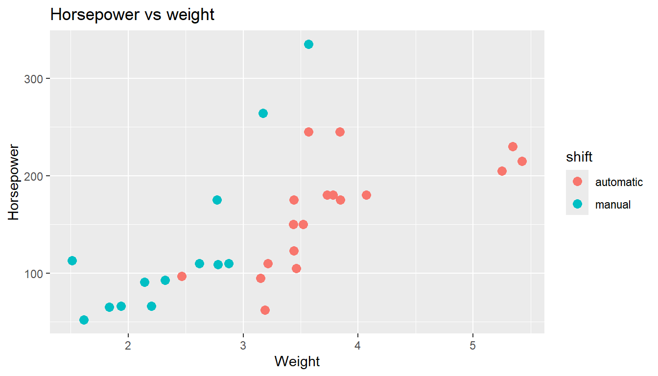

Add the code + geom_smooth(method = lm, se = FALSE) to the code above. Make sure that the “+” comes on the last line of existing code. Can you guess/describe what the new elements in the figure represents? (Don’t worry if you can’t, we will learn later anyway! :-))

Exercise 3.10 (Getting help) In this little exercise we try out some of R/Rstudio’s internal help tools, as well as external (web) sources. One should note that the internal guides in R are often somewhat compact and technical, while on the web you find more detailed examples.

Suppose we want to learn a bit about how R can help us do calculations with normal distributions. Suppose we have a standard normal variable \(Z\) and also another normal variable \(X\) with mean = 10, and standard deviation = 3.

We want to find out how we can find such things as \[P[Z \leq 2.1], P[Z \geq 2.1], P[X \leq 12], P[8.4 \leq X \leq 10.9].\]

Try to use the internal help system, via ?Normal or help(Normal) to find the probabilities. You should in this case not use standardization of \(X\) for the latter two cases, since there are built in general normal distributions in R.
See if you can find information about the same type of calculations via google (or similar). In fact, if you have access to some AI assistant like chatGPT or Copilot, this can be a very good place to ask R-related questions.
Proceed by internal or external help to find a number \(b\) such that \(P[Z \leq b] = 0.80\).
Can you also find a number \(c\) such that \(P[X \geq c] = 0.90\)?
Can you produce a vector my_x of 30 random numbers from the distribution of \(X\)? (The same normal distribution). Find the (sample) mean and standard deviation of my_x. Are they close to the real parameters?